Coefficient of Determination in Linear Regressions
Table of Contents
The coefficient of determinantion or r-squared value, which measures how good is the linear regression model, and the sums of squares are
defined and used to examine goodness of fit of the linear regressions. Examples and problems
with their solutions are also included.
Calculations of the coefficient of determinantion are done in details by steps using the formulas for the sums of squares and also using Excel for simple linear and also
multiple linear regression.
Errors in Mathematical Modelling
We start with the simple linear regression model where as shown below the dataset of ordred pairs \( \{(x_1,y_1) , (x_2,y_2), ... , (x_i,y_i) \} \) is modelled by \( \hat y = \hat \beta_1 x + \beta_0 \).
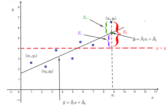
In accepting the model, we make an error \( E_e \) which is the difference between the measured value \( y_i \) and the \( \hat y_1 \) given by the regression model.
\( E_e = y_i - \hat y_i \) , where \( \hat y_i \) is the value of \( \hat y \) at \( x = x_i \)
The variations of the measured \( y_i \) value with respect to the mean \( \bar y \) of all values is given by
\( E_t = y_i - \bar y \)
wher \( \bar y \) is the mean of \( y_i \) value given by: \( \bar y = \dfrac{\sum_{i=1}^{m} y_i }{m} \) , \( m \) is the number of ordered pairs \( (x_i,y_i) \)
Because \( \hat y \) changes with \( x \), we define the error due to the variation of \( \hat y \) by
\( E_r = \hat y_i - \bar y \)
Note that \( E_t = E_e + E_r \)
Sums of Square Errors in Linear Regression
Assuming that we have \( m \) ordered pairs in the dataset, we now need to consider all ordered pairs \( (x_i,y_i) \) in the dataset in order to find the total errors. To find the total variations \( E_t \) defined above, We cannot for exammple just add all trems \( y_i - \bar y \) because
\( \sum_{i=1}^{m} ( y_i - \bar y ) = 0 \).
We therefore need to work with the squares of the errors \( E_e \), \( E_t \) and \( E_r \) defined above.
The sum of the square errors (SSE) due to \( E_e \) is defined by
\[ SSE = \sum_{i=1}^{m} (y_i - \hat y_i)^2 \]
We now define the total sum of squares (SST) due to \( E_t \) as the sum of the squares of the variations of the observed quantities \( y_i \) around their mean \( \bar y \) as follows:
\[ SST = \sum_{i=1}^{m} (y_i - \bar y)^2 \]
where \( \bar y \) is the mean of the observed values \( y_i \) defined above.
The regression sum of squares \( SSR \) due to \(E_r \) is defined by.
\[ SSR = \sum_{i=1}^{m} (\hat y_i - \bar y)^2 \]
In linear simple regressions, \( SST \) may be split into two terms
\[ SST = \sum_{i=1}^{m} (y_i - \bar y)^2 = \sum_{i=1}^{m} (y_i - \hat y_i)^2 + \sum_{i=1}^{m} (\hat y_i - \bar y)^2 \]
\[ SST = SSE + SSR \]
Coefficient of Determination
One of the most important question is how good is the regression linear model to represent the relationship between the dependent variable \( y \) and the independent variables \( x \)?
Let us define the coefficient of determination \( r^2 \) as
\[ r^2 = \dfrac{SSR}{SST} = 1 - \dfrac{SSE}{SST} \]
NOTE that
1 - the suggested linear regressions model is a good one if all ordered pairs in the dataset fall on or are close to the line given by the linear regression model. In this situation all the errors \(E_e \) defined in the graph above are close to zero therefore the square sum \( SSE \) of these errors approaches zero; hence \( r^2 \) approaches \( 1 \) or \( 100\% \).
2 - In other words, the coefficient of determination expresses the part (or percentage) of the variability of the values \( y_i \), in the dataset, that can be explained by the regression model of \( \hat y \) with \( x \).
3 - The sums of squares and the coefficient of determination formulas for multiple linear regression models are the same as the formulas given above except that the linear model is of the form: \( \hat y = \hat \beta_1 x_1 + \hat \beta_2 x_2 + ... + \beta_0 \).
Properties of the Coefficient of Determination in Linear Regression Models
1 - For linear regression models, the value of \( r^2 \) is in the interval \( [0, 1] \).
2 - When \( r^2 = 1\), the linear regression model suggested is perfect.
3 - In the case of a simple linear regression, the coefficient of determination is equal to the square of the correlation coefficient .
Examples with Solutions
Example 1
The table of values below shows measured data values of the dependent variable \( y \) and the independent variables \( x_1 \) and \( x_2\)
| \( x_1 \) | \(x_2\) | \(y\) |
|
| \( 0 \) | \( -1 \) | \( -1 \) |
| \( 2 \) | \( 2 \) | \( 4 \) |
| \( 6 \) | \( 5 \) | \( 7 \) |
| \( 7 \) | \( 10 \) | \( 8 \) |
| \( 8 \) | \( 11 \) | \( 9 \) |
a)
Assume that \( y \), \( x_1 \) and \( x_2 \) are related by
\( y = \beta_1 x_1 + \beta_2 x_2 + \beta_0 + \epsilon \) , where \( \epsilon \) is the error to minimize.
Use the normal equation to find \( \hat X = \begin{bmatrix}
\hat \beta_1\\
\hat \beta_2 \\
\hat \beta_0
\end{bmatrix} \) that minimizes the error \( \epsilon \) and hence write \( \hat y = \hat \beta_1 x_1 + \hat \beta_2 x_2 + \hat \beta_0 \)
b)
Find the sum of squares error \( SSE \) , the regression sum of squares \( SSR \) and the total sum of squares \( SST \) using their formulas given above and show that \( SST = SSE + SSR \).
c)
Find the coefficient of determination \( r^2 \) defined above.
d) Check your answer in parts a) and c) using Excel for multiple linear regression.
e) How good is the linear regression model used?
Solution to Example 1
a)
The mathematical model is of the from \( y = \beta_1 x_1 + \beta_2 x_2 + \beta_0 + \epsilon \) and therefore we use the method in multiple linear regression to find \( \hat X \).
Let
\( A = \begin{bmatrix}
0 & -1 & 1\\
2 & 2 & 1 \\
6 & 5 & 1 \\
7 & 10 & 1 \\
8 & 11 & 1
\end{bmatrix} \)
be the matrix of values, given in the table above, of the independent data variables \( x_1 \) and \( x_2 \) augmented by a colum of \( 1's \)
Let \( Y = \begin{bmatrix}
-1\\
4\\
7 \\
8 \\
9
\end{bmatrix} \) be a colum matrix of values , given in the table above, of the dependent variable \( y \)
Let \( X = \begin{bmatrix}
\beta_1\\
\beta_2 \\
\beta_0
\end{bmatrix} \) be a colum matrix of the factors involved in the linear model suggeted above.
The normal equation is given by
\[ \hat X = (A^T A)^{-1} A^T Y\]
The transpose \( A^T \) of matrix \( A \) is given by
\( A^T = \begin{bmatrix}
0 & 2 & 6 & 7 & 8\\
-1 & 2 & 5 & 10 & 11\\
1 & 1 & 1 & 1 & 1
\end{bmatrix} \)
The approximate solution \( \hat X \) is given by the normal equation
\( \hat X = \begin{bmatrix}
\hat \beta_1\\
\hat \beta_2\\
\hat \beta_0
\end{bmatrix} = (A^T A)^{-1} A^T Y
\\\\ = \left(
\begin{bmatrix}
0 & 2 & 6 & 7 & 8\\
-1 & 2 & 5 & 10 & 11\\
1 & 1 & 1 & 1 & 1
\end{bmatrix}
\begin{bmatrix}
\begin{bmatrix}
0 & -1 & 1\\
2 & 2 & 1 \\
6 & 5 & 1 \\
7 & 10 & 1 \\
8 & 11 & 1
\end{bmatrix}
\end{bmatrix} \right)^{-1}
\begin{bmatrix}
0 & 2 & 6 & 7 & 8\\
-1 & 2 & 5 & 10 & 11\\
1 & 1 & 1 & 1 & 1
\end{bmatrix}
\begin{bmatrix}
-1\\
4\\
7 \\
8 \\
9
\end{bmatrix} \\\\
= \begin{bmatrix}
\dfrac{112}{97}\\
-\dfrac{1}{97}\\
\dfrac{14}{97}
\end{bmatrix}
\approx \begin{bmatrix}
1.15463\\
-0.01031\\
0.144330
\end{bmatrix}
\)
b)
In what follows, \( \hat y_1, \hat y_2, ....\hat y_5 \) are the values of \( y \) calculated using the linear model and \( y_1, y_2, ....y_5 \) are the observed data values of the depenendent variable \( y \) given in the table of values.
Evaluate \( \hat y_1 \), \( \hat y_2 \), \( \hat y_3 \) , \( \hat y_4 \) and \( \hat y_5 \).
\( \hat y_1 = a_{1,1} \hat \beta_1 + a_{1,2} \hat \beta_2 + \hat \beta_0 = 0 \times \dfrac{112}{97} + (-1) \times (-\dfrac{1}{97}) + \dfrac{14}{97} = \dfrac{15}{97} \)
\( \hat y_2 = a_{2,1} \hat \beta_1 + a_{2,2} \hat \beta_2 + \hat \beta_0 = 2 \times \dfrac{112}{97} + 2 \times (-\dfrac{1}{97}) + \dfrac{14}{97} = 2\dfrac{42}{97} \)
\( \hat y_3 = a_{3,1} \hat \beta_1 + a_{3,2} \hat \beta_2 + \hat \beta_0 = 6 \times \dfrac{112}{97} + 5 \times (-\dfrac{1}{97}) + \dfrac{14}{97} = 7\dfrac{2}{97} \)
\( \hat y_4 = a_{4,1} \hat \beta_1 + a_{4,2} \hat \beta_2 + \hat \beta_0 = 7 \times \dfrac{112}{97} + 10 \times (-\dfrac{1}{97}) + \dfrac{14}{97} = 8\dfrac{12}{97} \)
\( \hat y_5 = a_{5,1} \hat \beta_1 + a_{5,2} \hat \beta_2 + \hat \beta_0 = 8 \times \dfrac{112}{97} + 11 \times (-\dfrac{1}{97}) + \dfrac{14}{97} = 9\frac{26}{97} \)
\( SSE = \sum_{i=1}^{5} (y_i - \hat y_i)^2 = (-1 - \dfrac{15}{97} )^2 + (4 - 2\dfrac{42}{97})^2 + (7 - 7\dfrac{2}{97})^2 + (8 - 8\dfrac{12}{97} )^2 + (9 - 9\frac{26}{97})^2 = 3\frac{85}{97} \)
Calculate the mean \( \bar y \)
\( \bar y = \dfrac{\sum_{i=1}^{5} y_i }{5} = \dfrac{-1+4+7+8+9}{5} = 5\frac{2}{5}\)
\( SST = \sum_{i=1}^{m} (y_i - \bar y)^2 = (-1 - 5\frac{2}{5} )^2 + (4 - 5\frac{2}{5} )^2 + (7 - 5\frac{2}{5})^2 +(8 - 5\frac{2}{5})^2 + (9 - 5\frac{2}{5})^2 = 65\frac{1}{5}\)
\( SSR = \sum_{i=1}^{m} (\hat y_i - \bar y)^2 = (\dfrac{15}{97} - 5\frac{2}{5} )^2 + (2\dfrac{42}{97} - 5\frac{2}{5} )^2 + ( 7\dfrac{2}{97} - 5\frac{2}{5})^2 +(8\dfrac{12}{97} - 5\frac{2}{5})^2 + (9\frac{26}{97} - 5\frac{2}{5})^2 = 61\frac{157}{485}\)
\( SSE + SSR = 3\frac{85}{97} + 61\frac{157}{485} = 65\dfrac{1}{5} = SST \)
c)
\( r^2 = 1 - \dfrac{SSE}{SST} = 1 - \dfrac{3\frac{85}{97}}{65\frac{1}{5}} = 0.9405\)
\( r^2 \) being close to \( 1 \) means that the modelling error \( SSE \) is much smaller than the total sum of squares \( SST \).
d)
Comparing \( r^2 = 0.9405\) calculated above in part c) with \( r^2 \) given by Excel as shown below, their values are very close.
Comparing \( \hat X = \begin{bmatrix}
\hat \beta_1\\
\hat \beta_2\\
\hat \beta_0
\end{bmatrix} = \approx \begin{bmatrix}
1.15463\\
-0.01031\\
0.144330
\end{bmatrix}
\) calculated above in part a) with those given by Excel and shown below, their values are very close; very small differences are due to rounding errors.
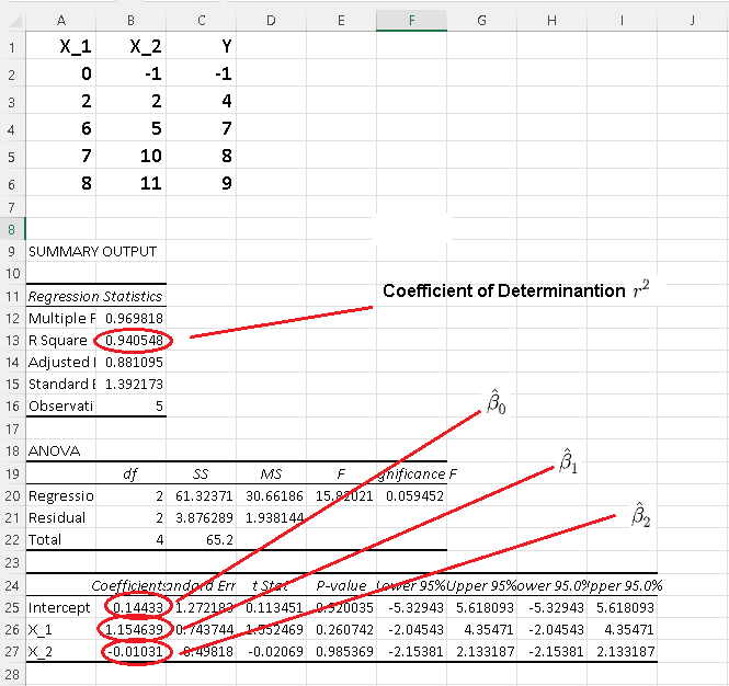
e) Since \( r^2 = 0.9405\) is close to 1, that means the sum of square errors SSE is close to zero and therefore the model is good. It also means that \( 95.05\% \) of the variability is due to the linear model \( \hat y = \hat \beta_1 x_1 + \hat \beta_2 x_2 + \hat \beta_0 \) used.
Problems with Solutions
Part A
The table of values below shows measured data values of the dependent variable \( y \) and the independent variables \( x_1 \), \( x_2\) and \( x_3 \)
| \( x_1 \) | \(x_2\) | \(x_3\) | \(y\) |
|
| \( 2 \) | \( 4 \) | \( 3 \) | \( -1 \) |
| \( 3 \) | \( 1 \) | \( 2 \) | \( 4 \) |
| \( 5 \) | \( 2 \) | \( 7 \) | \( 10 \) |
| \( 8 \) | \( -1 \) | \( 3 \) | \( 14\) |
| \( 12 \) | \( 10 \) | \( 4 \) | \( 15 \) |
a)
Assume that \( y \) and \( x_1 , x_2 \) and \( x_3 \) are related by
\( y = \beta_1 x_1 + \beta_2 x_2 + \beta_3 x_3 + \beta_0 + \epsilon\).
Use the normal equation to find \( \hat X = \begin{bmatrix}
\hat \beta_1\\
\hat \beta_2 \\
\hat \beta_3 \\
\hat \beta_0
\end{bmatrix} \) that minimizes \( \epsilon \) and hence write \( \hat y = \hat \beta_1 x_1 + \hat \beta_2 x_2 + \hat \beta_3 x_3 + \hat \beta_0 \).
b)
Find the sum of squares error \( SSE \) , the regression sum of squares \( SSR \) and the total sum of squares \( SST \) using their formulas given above and show that \( SST = SSE + SSR \).
c)
Find the coefficient of determination \( r^2 \) defined above.
d) Check your answer in parts a) and c) using Excel.
e) How good is the linear regression model used?
Part B
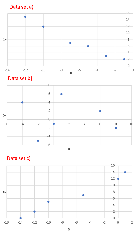
Give the datasets below
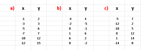
a) Make a scatter plot of all the three datasets and predict from these plot the datasets that may be modeled using a linear regression mdel.
b) Use Excel to find the coefficient of determination of each data set and explain for which dataset(s) would a linear regression model be a good one?
Solutions to the Above Problems
Part A
a)
The mathematical model is of the from \( y = \beta_1 x_1 + \beta_2 x_2 + \beta_3 x_3 + \beta_0 + \epsilon \)
Let
\( A = \begin{bmatrix}
2 & 4 & 3 & 1\\
3 & 1 & 2 & 1 \\
5 & 2 & 7 & 1 \\
8 & -1 & 3 & 1 \\
12 & 10 & 4 & 1
\end{bmatrix} \)
be the matrix of values, given in the table above, of the independent data variables \( x_1 \) and \( x_2 \) augmented by a colum of \( 1's \)
Let \( Y = \begin{bmatrix}
-1\\
4\\
10 \\
14 \\
15
\end{bmatrix} \) be a colum matrix of values , given in the table above, of the dependent variable \( y \)
Let \( X = \begin{bmatrix}
\beta_1\\
\beta_2 \\
\beta_3 \\
\beta_0
\end{bmatrix} \) be a colum matrix of the factors involved in the linear model suggeted above.
The normal equation is given by
\[ \hat X = (A^T A)^{-1} A^T Y\]
The transpose \( A^T \) of matrix \( A \) is given by
\( A^T = \begin{bmatrix}
2 & 3 & 5 & 8 & 12\\
4 & 1 & 2 & -1 & 10\\
3 & 2 & 7 & 3 & 4 \\
1 & 1 & 1 & 1 & 1
\end{bmatrix} \)
The approximate solution \( \hat X \) is given by the normal equation
\( \hat X = \begin{bmatrix}
\hat \beta_1\\
\hat \beta_2\\
\hat \beta_3\\
\hat \beta_0
\end{bmatrix} = (A^T A)^{-1} A^T Y
= \begin{bmatrix}
1.8560\\
-0.7093 \\
0.7500 \\
-3.3159
\end{bmatrix}
\)
b)
\( \hat Y = \begin{bmatrix} \hat y_1 \\ \hat y_2\\ \hat y_3\\ \hat y_4\\ \hat y_5 \end{bmatrix} = A \hat X = \begin{bmatrix}-0.19144\\ 3.04264\\ 9.795\\ 14.49126\\ 14.86246\end{bmatrix} \)
\( Y - \hat Y = \begin{bmatrix} -0.80856 \\
0.95736 \\
0.205 \\
-0.49126 \\
0.13754
\end{bmatrix}
\)
\( SSE = ( -0.80856)^2 + 0.95736^2 + 0.205^2 + (-0.49126)^2 + 0.13754^2 = 1.87258 \)
\(\bar y = \dfrac{-1+4+10+14+15}{5} = 8.4\)
\( SST = \sum_{i=1}^5 (y_i - 8.4)^2 = (-9.4)^2 + (-4.4)^2 + 1.6^2 + 5.6^2 + 6.6^2 = 185.2 \)
\( SSR = \sum_{i=1}^5 (\hat y_i - 8.4)^2 = (-0.19144 - 8.4)^2 + (3.04264 - 8.4)^2 + (9.795 - 8.4)^2 + (14.49126 - 8.4)^2 + (14.86246 - 8.4)^2 = 183.32 \)
\( SSE + SSR = 1.87258 + 183.32 = 185.19258 \approx SST \)
c)
\( r^2 = 1 - \dfrac{SSE}{SST} = 1 - \dfrac{1.87258}{185.2 } = 0.98988 \)
\(r^2 \) is close to \( 1 \) which indicates that the model used is a good fit to the given data.
d)
\( r^2 = 0.98988\) calculated above in part c) with \( r^2 \) given by Excel as shown below are very close.
The very small differences between \( \hat X = \begin{bmatrix}
\hat \beta_1\\
\hat \beta_2\\
\hat \beta_3\\
\hat \beta_0
\end{bmatrix} = \approx \begin{bmatrix}
1.8560\\
-0.7093 \\
0.7500 \\
-3.3159
\end{bmatrix}
\) calculated above in part a) and those given by Excel and shown below are due to rounding errors.
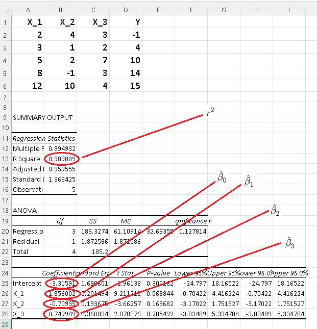
e) Since \( r^2 = 0.98988\) is close to 1, the suggested linear model is very good.
Part B
a)
Scatter plots of all three datasets given are shown below. Since the scatter plots in the datasets a) and c) are close to linear, we would expect that a simple linear regression model would be good for these two datasets.
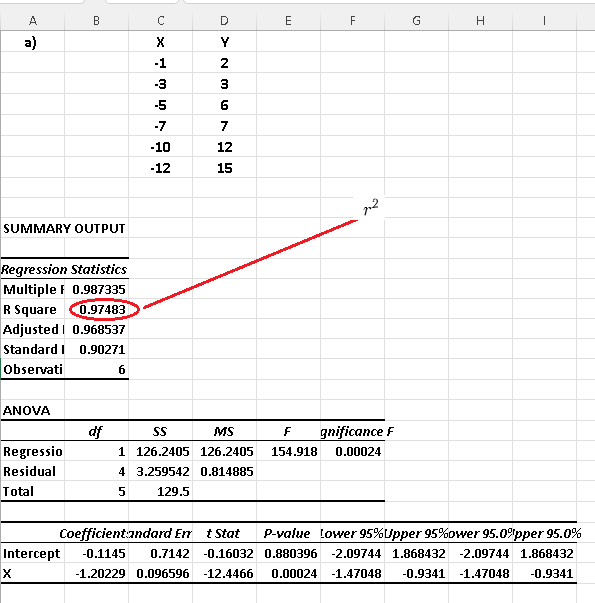
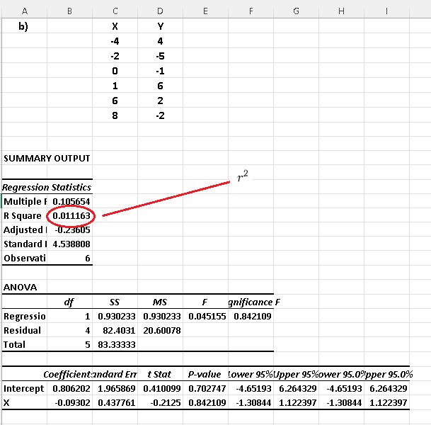
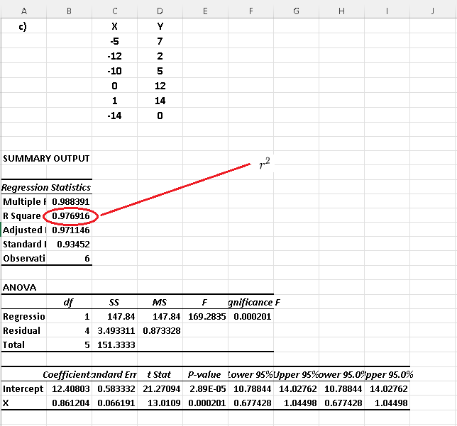
b)
Using Excel linear regression steps, we have the results below for each dataset.
As already predicted from the scatter plots, datasets a) and c) have the coefficients of determination close to 1 and therefore the use of linear regression to model the datasets in a) and c) would be appropriate.
More References and links
- Multiple Linear Regression
- Simple Linear Regression
- Simple Linear Regression Examples with Real Life Data
- Correlation Coefficient
- Simple Linear Regression Using Excel
- Multiple Linear Regression Using Excel
- Matrices