Multiple Linear Regression With Examples
Table of Contents
The ordinary least squares (OLS) regression [1] method is presented with examples and problems with their solutions.
As a practical example, The North American Datum of 1983 (NAD 83), used the least square method to solve a system which involved 928,735 equations with 928,735 unknowns [2] which is in turn used in global positioning systems (GPS).
Least square linear regression is also used in business and finance to make predictions [5].
Ordinary Least Square Regression
Let us assume that in the table below is shown observed or measured data values of the dependent variable \( y \) related to the \( n \) independent observed or measured variables \( x_1, x_2 , ..., x_n \)
| \( x_1 \) | \(x_2\) | ... | \(x_n\) | \(y\) |
|
| \(a_{1,1} \) | \(a_{1,2} \) | ... | \(a_{1,n} \) | \(y_1 \) |
| \(a_{2,1} \) | \(a_{2,2}\) | ... | \(a_{2,n} \) | \(y_2 \) |
| ... | ... | ... | ... | ... |
| ... | ... | ... | ... | ... |
| \(a_{m,1} \) | \(a_{m,2} \) | ... | \(a_{m,n} \) | \(y_m \) |
A possible linear mathematical model or equation relating \( y \) to \( x_1, x_2 , ..., x_n \) may be written in the form
\[ y = \beta_1 x_1 + \beta_2 x_2 + ... + \beta_n x_n + \beta_0 + \epsilon \]
where \( \epsilon \) is an error.
We also assume that the observed data values follow the same model as follows
\( y_1 = \beta_1 a_{1,1} + \beta_2 a_{1,2} + ... + \beta_n a_{1,n} + \beta_0 + \epsilon_1 \quad (I) \\
y_2 = \beta_1 a_{2,1} + \beta_2 a_{2,2} + ... + \beta_n a_{2,n} + \beta_0 + \epsilon_2 \\
. . . \\
y_m = \beta_1 a_{m,1} + \beta_2 a_{m,2} + ... + \beta_n a_{m,n} + \beta_0 + \epsilon_m \)
Question: Find the coefficients \( \beta_1, \beta_2, ...., \beta_n , \beta_0 \) that minimize the error \( \epsilon \).
Let \( Y \) be a column matrix of dimension \( n \times 1 \) representing observed or measured values of the dependent variable \( y \) and matrix \( A \) of dimension \( m \times (n + 1) \) the observed or measured values of \( n \) independent variables.
\( A = \begin{bmatrix}
a_{1,1} & a_{1,2} & ... & a_{1,n} & 1 \\
a_{2,1} & a_{2,2} & ... & a_{2,n} & 1 \\
... & ... & ... & ... & \\
a_{m,1} & a_{m,2} & ... & a_{m,n} & 1
\end{bmatrix}
\)
, \( X = \begin{bmatrix}
\beta_{1}\\
\beta_{2}\\
... \\
\beta_{n} \\
\beta_0
\end{bmatrix}
\)
and
\( Y = \begin{bmatrix}
y_{1}\\
y_{2}\\
... \\
y_{m}
\end{bmatrix}
\)
Note a column of \(1's\) have been added to the matrix of the independent data values \( x_i \) to account for the intercept \( \beta_0 \).
The system of equations (I) above may be now be written in matrix form as follows
\[ Y = A X + \epsilon \quad (I) \]
with \( \epsilon = \begin{bmatrix}
\epsilon_{1}\\
\epsilon_{2}\\
... \\
\epsilon_{m}
\end{bmatrix}
\) being an \( m \times 1 \) matrix of random errors.
Matrix \( A \) has the dimension \( m \times (n+1) \) and \( Y \) is a column matrix of dimension \( m \)
much larger than \( n \).
Such a system of equations may not have an exact solution since the number of equations \( m \) is much larger than the number of the unknowns \( n \) and therefore the need for an approximate solution.
In practice, matrices \( A \) and \( Y \) may have large dimensions, sometimes in the millions, and we need to find approximate a solution \( \hat X = \begin{bmatrix}
\hat \beta_{1}\\
\hat \beta_{2}\\
... \\
\hat \beta_{n} \\
\hat \beta_0
\end{bmatrix}
\) that minimizes the norm or length of the error \( \epsilon = AX - Y \).
The least square method is used to find the values of the parameters \( \hat \beta_{0}, \hat \beta_{1}, \hat \beta_2 ,..., \hat \beta_{n} \) that minimizes the square of the norm or length of vector \( \epsilon = A X - Y \).
Because the norm involves the square root function, for practical reasons and to avoid dealing with the square roots in our calculations, we minimize the square of the norm instead the norm.
Note that \( \; A X - Y \; \) is a column matrix and therefore we express its norm as follows:
\[ || A X - Y ||^2 = ( A X - Y )^T ( A X - Y )\]
where \( ( A X - Y )^T \) is the matrix transpose of the column matrix \( A X - Y \)
The least square method is based on the idea of finding the vector \( X \) that minimizes \( || \epsilon(\hat \beta_{1}, \hat \beta_2 ,..., \hat \beta_{n}, \hat \beta_{0}) ||^2 = || A X - Y ||^2 \)
We first substitute \(A\), \( X \) and \( Y \) by their definitions given above.
\( \epsilon = A X - Y =
\begin{bmatrix}
\sum_{i=1}^{n} a_{1,i} \beta_i + \beta_0 - y_1\\
...\\
... \\
\sum_{i=1}^{n} a_{m,i} \beta_i + \beta_0 - y_m
\end{bmatrix}
\)
Hence we have
\( \displaystyle || \epsilon(\hat \beta_{1}, \hat \beta_2 ,..., \hat \beta_{n}, \hat \beta_{0}) ||^2 = \sum_{j=1}^{m} \left(\sum_{i=1}^{n} a_{j,i} \beta_i+ \beta_0- y_j \right)^2 \quad (I) \)
The above is a function of the variables \( \beta_1, \beta_2, ..., \beta_n, \beta_0\) with \( n \) partial derivatives given by
\( \displaystyle \dfrac{ \partial \epsilon(\beta_1, \beta_2 ... \beta_n, \beta_0)}{\partial \beta_i} = 2 \sum_{j=1}^{m} a_{i,j} ( \sum_{i=1}^{n} a_{j,i} \beta_i + \beta_0 - y_j) \) for \( i = 1, ..., n \)
\( \displaystyle \dfrac{ \partial \epsilon(\beta_1, \beta_2 ... \beta_n, \beta_0)}{\partial \beta_0} = 2 \sum_{j=1}^{m} ( \sum_{i=1}^{n} a_{j,i} \beta_i + \beta_0- y_j) \)
which in vector form may be written as the gradient of \( || \epsilon(\hat \beta_{1}, \hat \beta_2 ,..., \hat \beta_{n}, \hat \beta_{0}) ||^2 \) as follows
\( \displaystyle \nabla || \epsilon(\hat \beta_{1}, \hat \beta_2 ,..., \hat \beta_{n}, \hat \beta_{0}) ||^2 =
\begin{bmatrix}
\dfrac{ \partial \epsilon(X)}{\partial \beta_1}\\
...\\
... \\
\dfrac{ \partial \epsilon(X)}{\partial \beta_n} \\
\dfrac{ \partial \epsilon(X)}{\partial \beta_0}
\end{bmatrix}
=
\begin{bmatrix}
2 \sum_{j=1}^{m} a_{j,1}( \sum_{i=1}^{n} a_{j,1} \beta_1 + \beta_0 - y_j)\\
...\\
... \\
2 \sum_{j=1}^{m} a_{j,n} ( \sum_{i=1}^{n} a_{j,n} \beta_n + \beta_0 - y_j) \\
2 \sum_{j=1}^{m} ( \sum_{i=1}^{n} a_{j,n} \beta_n + \beta_0 - y_j)
\end{bmatrix} = 2 A^T (A X - Y)
\)
The norm \( || \epsilon(\hat \beta_{1}, \hat \beta_2 ,..., \hat \beta_{n}, \hat \beta_{0}) ||^2 \) has a minimum value when \( \displaystyle\nabla || \epsilon(\hat \beta_{1}, \hat \beta_2 ,..., \hat \beta_{n}, \hat \beta_{0}) ||^2 = 0 \) [3] which gives
\[ A^T (A \hat X - Y) = 0 \]
which may be written as
\[ A^T A \hat X = A^T Y \]
Multiply both sides by the inverse of the matrix \( (A^T A)^{-1} \) and simplify to obtain the normal equation
\[ \hat X = (A^T A)^{-1} A^T Y \quad (II)\]
Notes
1) The above solution holds when the inverse matrix \( (A^T A)^{-1} \) exists in other words when the columns of \( Y \) are linearly independent [4].
2) The extrema at \( X = \hat X \) is a minimum because of the quadratic terms in the expression of \( \epsilon\) in (I).
3) Although the matrices involved may have large dimensions, computers may be used to solve efficiently the normal equation (II) found above.
Examples with Solutions
Example 1
Let \( A = \begin{bmatrix}
1 & 1 \\
2 & 1\\
4 & 1
\end{bmatrix} \) , \( Y = \begin{bmatrix}
0\\
4\\
7
\end{bmatrix} \) and \( X = \begin{bmatrix}
\beta_1\\
\beta_0
\end{bmatrix} \)
a)
Express \( || \epsilon(\beta_{1}, \beta_{0}) ||^2 = ( A X - Y )^T ( A X - Y ) \) in terms of \( \beta_1 \) and \( \beta_0 \).
b)
Find the solution \( \hat X \begin{bmatrix}
\hat \beta_1\\
\hat \beta_0
\end{bmatrix} \) that minimizes \( || \epsilon(\beta_{1}, \beta_{0}) ||^2 \) using the normal equation \( \hat X = (A^T A)^{-1} A^T Y \).
c)
Graph \( || \epsilon(\beta_{1}, \beta_{0}) ||^2 ) \) and show that it has a minimum at \( \hat X = \begin{bmatrix}
\hat \beta_1\\
\hat \beta_0
\end{bmatrix} \) found in par b).
d) Use any software to calculate the vector \( \hat X \begin{bmatrix}
\hat \beta_1\\
\hat \beta_0
\end{bmatrix} \) and compare with the results obtained in part b).
Solution to Example 1
a)
\( ( A X - Y ) = \begin{bmatrix}
1 & 1 \\
2 & 1\\
4 & 1
\end{bmatrix} \begin{bmatrix}
\beta_1\\
\beta_0
\end{bmatrix} - \begin{bmatrix}
0\\
4\\
7
\end{bmatrix} \\\\
\quad =
\begin{bmatrix}
\beta_1 + \beta_0 \\
2 \beta_1 + \beta_0 - 4\\
4 \beta_1 + \beta_0 - 7
\end{bmatrix}
\)
\( || \epsilon( \beta_{1}, \beta_{0}) ||^2 = ( A X - Y )^T ( A X - Y ) \\ = (\beta_1 + \beta_0)^2 + (2 \beta_1 + \beta_0 - 4)^2 + (4 \beta_1 + \beta_0 - 7)^2 \)
b)
The transpose \( A^T \) of matrix \( A \) is given by
\( A^T = \begin{bmatrix}
1 & 2 & 4 \\
1 & 1 & 1
\end{bmatrix} \)
\( (A^T A)^{-1}
= \left(\begin{bmatrix}
1 & 2 & 4 \\
1 & 1 & 1
\end{bmatrix} \begin{bmatrix}
1 & 1 \\
2 & 1\\
4 & 1
\end{bmatrix} \right)^{-1} = \begin{bmatrix}
\dfrac{3}{14}&-\dfrac{1}{2}\\
-\dfrac{1}{2}&\dfrac{3}{2}
\end{bmatrix}
\)
The approximate solution is given by
\( \hat X = (A^T A)^{-1} A^T Y \)
Substitute by the known quantities to obtain
\( \hat X = \begin{bmatrix}
\dfrac{3}{14}&-\dfrac{1}{2}\\
-\dfrac{1}{2}&\dfrac{3}{2}
\end{bmatrix} \begin{bmatrix}
1 & 2 & 4 \\
1 & 1 & 1
\end{bmatrix} \begin{bmatrix}
0\\
4\\
7
\end{bmatrix} \)
Evaluate
\( \hat X = \begin{bmatrix}
\hat \beta_1\\
\hat \beta_0
\end{bmatrix} =
\begin{bmatrix}
\dfrac{31}{14}\\
-\dfrac{3}{2}
\end{bmatrix} \approx
\begin{bmatrix}
2.21\\
-1.5
\end{bmatrix}
\)
c)
\(|| \epsilon( \hat \beta_{1}, \hat \beta_{0}) ||^2 \\
= ( \hat \beta_1 + \hat \beta_0)^2 + (2 \hat \beta_1 + \hat \beta_0 - 4)^2 + (4 \hat \beta_1 + \hat \beta_0 - 7)^2 \\
= \left( \dfrac{31}{14} -\dfrac{3}{2} \right)^2 + \left(2 \times \dfrac{31}{14} -\dfrac{3}{2} - 4 \right)^2 + \left(4 \times \dfrac{31}{14} -\dfrac{3}{2} - 7\right)^2 \\
= \dfrac{25}{14} \approx 1.79
\)
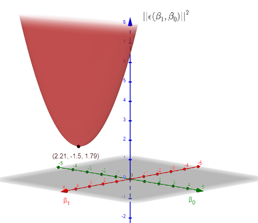
The graph of \( || \epsilon( \beta_{1}, \beta_{0}) ||^2 \) is shown below. It has a minimum at point \( M = (2.21,-1.5,1.79) \).
The minimum value of \( |||| \epsilon( \beta_{1}, \beta_{0}) ||^2 \) is approximately equal to \( 1.79 \) at \( X = \begin{bmatrix}
\beta_1\\
\beta_0
\end{bmatrix} \approx \begin{bmatrix}
2.21\\
-1.5
\end{bmatrix} \) as predicted in the analytical calculations above.
d)
Using for multiple linear regression , we obtain the results shown in the table which are exactly the results obtained in the detailed calculations of parts b) above.
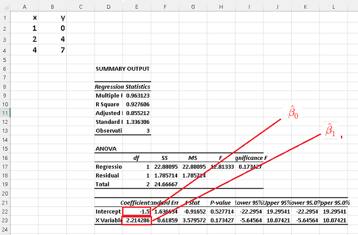
You may use the online multiple linear regression calculator to check the answers to the examples and problems.
Problems with Solutions
Part A
Given the data sets below:
a) Find a least square solution \( \hat X = (A^T A)^{-1} A^T Y \) using the steps as in example 1
b) Use any software to calculate \( \hat X = (A^T A)^{-1} A^T Y \) and compare the results.
1)
\( A = \begin{bmatrix}
-1 & 1 \\
1 & 1\\
2 & 1\\
3 & 1
\end{bmatrix} \) , \( Y = \begin{bmatrix}
4\\
8\\
10\\
12
\end{bmatrix} \)
2)
\( A = \begin{bmatrix}
-1 & -1 & 1\\
0 & 3 & 1\\
2 & 5 & 1\\
4 & 9 & 1
\end{bmatrix} \) , \( Y = \begin{bmatrix}
-4\\
6\\
7\\
10
\end{bmatrix} \)
Part B
A company spends an amount \( x_1 \) on advertising and an amount \( x_2 \) on improving the quality of its product. The profit \( y \) over a period of 5 months is given in the table below. \( x_1, x_2 \) and \( y \) are in millions of dollars.
| \( x_1 \) | \(x_2\) | \(y\) |
|
| \( 2 \) | \( 1.5 \) | \( 3 \) |
| \( 2.5 \) | \( 1.7 \) | \( 3.2 \) |
| \( 3.0\) | \( 1.8 \) | \( 3.5 \) |
| \( 3.2\) | \( 2.1 \) | \( 4.1\) |
| \( 3.4 \) | \( 2.5 \) | \( 4.6\) |
Use a linear model of the form \( y = \beta_1 x_1 + \beta_2 x_2 + \beta_0 + \epsilon\) to approximate the profit for \( x_1 = 4 \) and \( x_2 = 4 \) (in millions of dollars)
Solutions to the Above Problems
Part A
1)
a)
\( A^T = \begin{bmatrix}
-1 & 1 & 2 & 3 \\
1 & 1 & 1 & 1
\end{bmatrix}
\)
\( A^T A = \begin{bmatrix}
-1 & 1 & 2 & 3 \\
1 & 1 & 1 & 1
\end{bmatrix}
\begin{bmatrix}
-1 & 1 \\
1 & 1\\
2 & 1\\
3 & 1
\end{bmatrix}
=
\begin{bmatrix}
15 & 5\\ 5 & 4
\end{bmatrix}
\)
\( (A^T A)^{-1} =
\begin{bmatrix}
\dfrac{4}{35}&-\dfrac{1}{7}\\
-\dfrac{1}{7}&\dfrac{3}{7}
\end{bmatrix}
\)
\( \hat X = (A^T A)^{-1} A^T Y = \begin{bmatrix}
\hat \beta_1\\
\hat \beta_0
\end{bmatrix}
= \begin{bmatrix}
2\\
6
\end{bmatrix}
\)
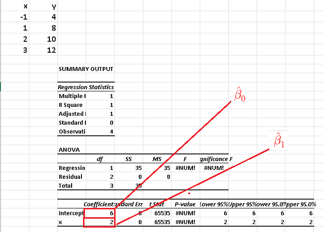
b)
The use of Excel for multiple linear regression , we obtain the results shown in the table which are exactly the results obtained in the detailed calculations of parts b) above.
2)
a)
\begin{bmatrix}
-1 & -1 & 1\\
0 & 3 & 1\\
2 & 5 & 1\\
4 & 9 & 1
\end{bmatrix}
\( A^T =
\begin{pmatrix}
-1&0&2&4\\
-1&3&5&9\\
1&1&1&1
\end{pmatrix}
\)
\( A^T A =
\begin{pmatrix}
-1&0&2&4\\
-1&3&5&9\\
1&1&1&1
\end{pmatrix}
\begin{bmatrix}
-1 & -1 & 1\\
0 & 3 & 1\\
2 & 5 & 1\\
4 & 9 & 1
\end{bmatrix} =
\begin{bmatrix}
21&47&5\\
47&116&16\\
5&16&4
\end{bmatrix}
\)
\( (A^T A)^{-1} =
\begin{bmatrix}
\dfrac{26}{19}&-\dfrac{27}{38}&\dfrac{43}{38}\\ -\dfrac{27}{38}&\dfrac{59}{152}&-\dfrac{101}{152}\\ \dfrac{43}{38}&-\dfrac{101}{152}&\dfrac{227}{152}
\end{bmatrix}
\)
\( \hat X = (A^T A)^{-1} A^T Y
= \begin{bmatrix}
\hat \beta_1\\
\hat \beta_2\\
\hat \beta_0
\end{bmatrix}
=
\begin{bmatrix}
-\dfrac{68}{19}\\ \dfrac{245}{76}\\ -\dfrac{279}{76}
\end{bmatrix}
\approx
\begin{bmatrix}
-3.57894 \\ 3.22368\\ - 3.67105
\end{bmatrix}
\)
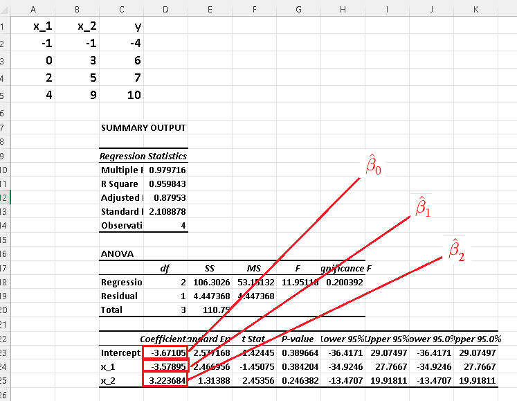
b)
Using Excel for multiple linear regression , we obtain the results shown in the table which are exactly the results obtained in the detailed calculations of parts b) above.
Part B
Let \( A =
\begin{bmatrix}
2 & 1.5 & 1\\
2.5 & 1.7 & 1\\
3.0 & 1.8 & 1\\
3.2 & 2.1 & 1\\
3.4 & 2.5 & 1
\end{bmatrix}
\) and \( Y =
\begin{bmatrix}
3.0\\
3.2\\
3.5\\
4.1\\
4.6
\end{bmatrix}
\)
Hence
\( A^T = \begin{bmatrix}
2 & 2.5 & 3.0 & 3.2 & 3.4\\
1.5 & 1.7 & 1.8 & 2.1& 2.5\\
1 & 1 & 1 & 1 & 1
\end{bmatrix}
\)
\( A^T A =
\begin{bmatrix}
2 & 2.5 & 3.0 & 3.2 & 3.4\\
1.5 & 1.7 & 1.8 & 2.1& 2.5\\
1 & 1 & 1 & 1 & 1
\end{bmatrix}
\begin{bmatrix}
2 & 1.5 & 1\\
2.5 & 1.7 & 1\\
3.0 & 1.8 & 1\\
3.2 & 2.1 & 1\\
3.4 & 2.5 & 1
\end{bmatrix} \\
=
\begin{bmatrix}
41.05&27.87&14.1\\
27.87&19.04&9.6\\
14.1&9.6&5
\end{bmatrix}
\)
\( (A^T A)^{-1} =
\begin{bmatrix}
4.15584 &-5.45454 &-1.24675 \\ -5.45454 &8.80382 &-1.52153 \\ -1.24675 &-1.52153 &6.63718
\end{bmatrix}
\)
\( \hat X = \begin{bmatrix}
\hat \beta_1 \\ \hat \beta_2 \\ \hat \beta_0
\end{bmatrix} \\
\quad = (A^T A)^{-1} A^T Y \\
\quad =
\begin{bmatrix}
0.1273094\\
1.5139046\\
0.4145915
\end{bmatrix}
\)
Hence
\( \hat y = 0.1273094 x_1 + 1.5139046 x_2 + 0.4145915 \)
Prediction
\( \hat y = 0.1273094 \times 4 + 1.5139046 \times 4 + 0.4145915 = 6.9794475 \) (in millions of dollars)
More References and links
- Mansfield Merriman, "A List of Writings Relating to the Method of Least Squares"
- North American Datum of 1983, Charles R. Schwarz (ed.), National Geodetic Survey, National Oceanic and Atmospheric Administration (NOAA) Professional Paper NOS 2, 1989.
- Anton's Calculus: Early Transcendentals, 11th Edition, Global Edition - Howard Anton, Irl C. Bivens, Stephen Davis - ISBN: 978-1-119-24890-3
- Stock Market Price Prediction Using Linear and Polynomial Regression Models- Semantic Scholar - 2014
- Inverse of a Matrix
- Matrices
- Systems of Equations
- Simple Linear Regression Examples with Real Life Data
- Multiple Linear Regression Using Excel.
- Multiple Linear Regression Calculator