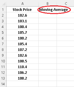
Step 2 - Create a label for the moving average outputs in a column adjacent to the given data.
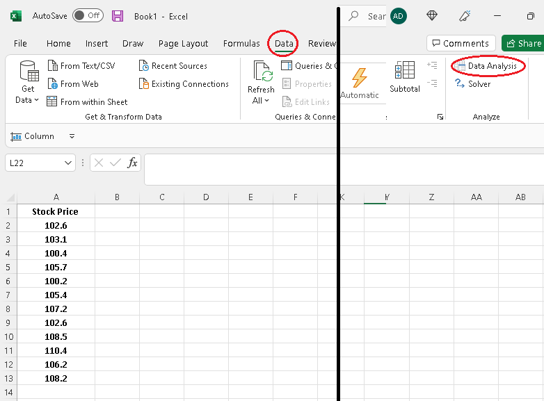
Step 3 - Press on the "Data" tab and click on "Data Analysis".
Step 4 - Select "Moving Average" and press "OK".

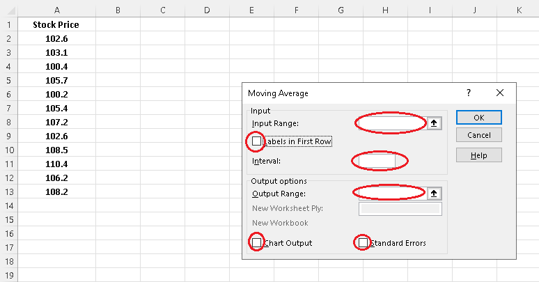
Step 5 - Clear all inputs and output areas.
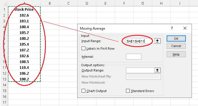
Step 6 - Click inside "Input Range" and use the mousse to select the column containing the data values, whose moving average you need to calculate, including the label "Stock Price".
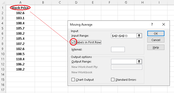
Step 7 - Check labels because you included the label when selecting the input data in step 6.
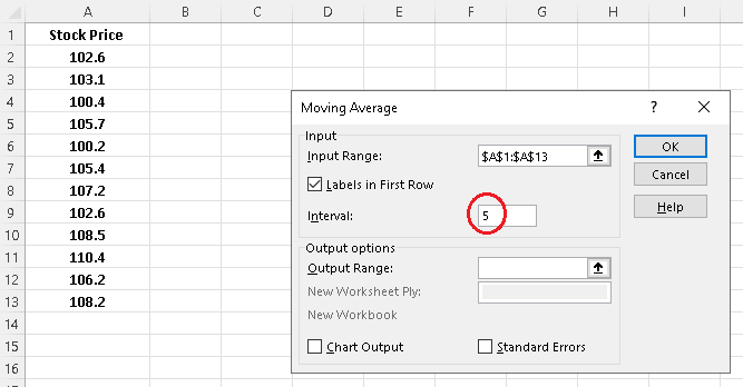
Step 8 - Input the interval of the moving average to be calculated. In this example we are looking for the 5-day moving average, therefore the interval is 5
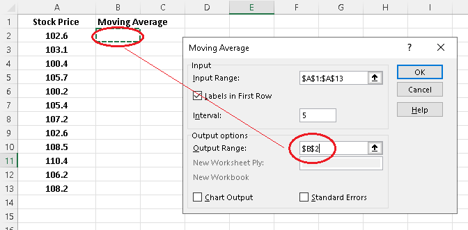
Step 9 - Click inside "Output Range" and use mousse to select the first cell below the label "Moving Average".
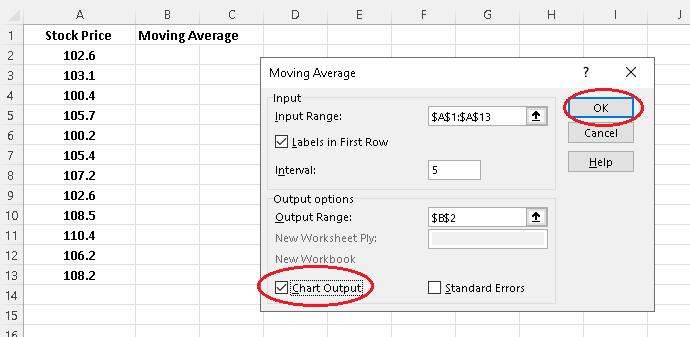
Step 10 - Check "Chart Output" and press OK.
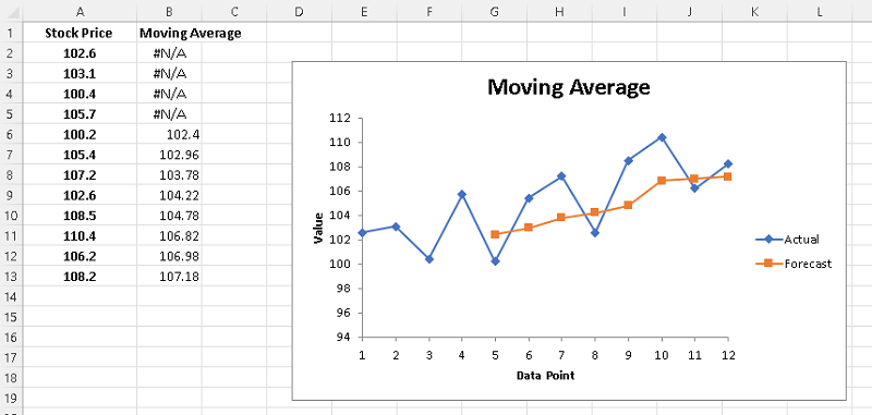
Step 11 - Read and interpret the data and the graphs. The moving average is in column "Moving Average" and start on day 5. You also have the graphs of both the stock prices and the 5-day moving average on the same system of axes which you can format the way you wish.