Moving Average of Real Life Data
Table of Contents
The concept of moving average and its properties are presented with examples using real life data and their solutions.
The moving average in example 2 is calculated by hand in order to understand the its meaning. Then the steps in moving average using Excel are used for more example with extensive real life data.
The Average
The average of a set of data values is the sum of the data values divided by the number of data values. [1] [2] [3] [4].
Let \( \{ x_1, x_2, ..., x_n \} \) be data values.
The average \( a \) of the sample is given by
\[ a = \dfrac{\sum_{i=1}^n x_i}{n} \]
Example 1
Find the average \( a \) of the data values in the set \( -1.4 , 8.3 , 9 , -10.2 , 13 , 40 , -16, 74 , -92 , 12.4 \)
Solution to Example 1
There are 10 data values in the given set, hence \( n = 10 \)
\( a = \dfrac{-1.4 + 8.3 + 9 -10.2 + 13 + 40 -16 + 74 -92 + 12.4}{10} = 3.71\)
The Moving Average
The moving average of a time series is an average of a fixed number of observations (subset) [1] that moves as time increases.
For stock prices for example, the subset whose average is calculated starts from the initial obseravation and progesses in time. The subset can have any number of observations; 5 for example which we call a 5 day moving average.
Example 2
The stock prices, in dollars, of a company over a period of 12 days are given below.
\( 102.6 , 103.1 , 100.4 , 105.7 , 100.2 , 105.4 , 107.2 , 102.6 , 108.5 , 110.4 , 106.2 , 108.2\)
a) Find the 5-days moving average of the stock price given above and organize in a table.
b) Use line graphs to graph the stock price and its 5 days moving average on the same system of axes.
Solution to Example 2
a)
Step 1: Find the average \( a_1 \) from day 1 to day 5 (5 days) using the corresponding stock prices: \( 102.6 , 103.1 , 100.4 , 105.7 , 100.2 \)
\( a_1 = \dfrac{102.6 + 103.1 + 100.4 + 105.7 + 100.2}{5} = 102.4 \)
Step 2: Find the average \( a_2 \) from day 2 to day 6 (5 days) using the corresponding stock prices: \( 103.1 , 100.4 , 105.7 , 100.2, 105.4 \)
\( a_2 = \dfrac{103.1 + 100.4 + 105.7 + 100.2+105.4}{5} = 102.96 \)
Step 3: Find the average \( a_3 \) from day 3 to day 7 (5 days) using the corresponding stock prices: \( 100.4 , 105.7 , 100.2, 105.4 , 107.2\)
\( a_3 = \dfrac{100.4 + 105.7 + 100.2+105.4 + 107.2}{5} = 103.78 \)
Step 4: Find the average \( a_4 \) from day 4 to day 8 (5 days) using the corresponding stock prices: \( 105.7 , 100.2, 105.4 , 107.2 , 102.6\)
\( a_4 = \dfrac{105.7 + 100.2+105.4 + 107.2+102.6}{5} = 104.22 \)
Step 5: Find the average \( a_5 \) from day 5 to day 9 (5 days) using the corresponding stock prices: \( 100.2, 105.4 , 107.2 , 102.6 , 108.5\)
\( a_5 = \dfrac{100.2+105.4 + 107.2+102.6+108.5}{5} = 104.78 \)
Step 6: Find the average \( a_6 \) from day 6 to day 10 (5 days) using the corresponding stock prices: \( 105.4 , 107.2 , 102.6 , 108.5 , 110.4\)
\( a_6 = \dfrac{105.4 + 107.2+102.6+108.5+110.4}{5} = 106.82 \)
Step 7: Find the average \( a_7 \) from day 7 to day 11 (5 days) using the corresponding stock prices: \( 107.2 , 102.6 , 108.5 , 110.4 , 106.2\)
\( a_7 = \dfrac{107.2+102.6+108.5+110.4+106.2}{5} = 106.98 \)
Step 8: Find the average \( a_7 \) from day 8 to day 12 (5 days) using the corresponding stock prices: \( 102.6 , 108.5 , 110.4 , 106.2 , 108.2\)
\( a_8 = \dfrac{102.6+108.5+110.4+106.2+108.2}{5} = 107.18 \)
The 5 days moving average of the given stock prices, starting from day 5, is given by the set of values : \( 102.4 , 102.96 , 103.78 , 104.22 , 104.78 , 106.82 , 106.98 , 107.18 \)
and may be organized in a table as follows:
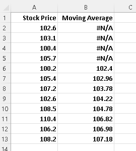
Note that because we are looking for the 5-day moving average and we therefore need 5 days, we only start calculating the moving average on day 5; hence the "#N/A" (not available) in the first 4 days of the moving average column.
b)
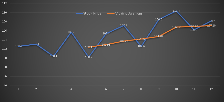
The graphs of the stock price and its 5-day moving average are shown below. The graphs of the stock price shows large variations while the 5-day moving average graph is smoother but clearly shows the upward trend of the stock price over the period of 12 days.
The moving average smoothes out the main data (the stock price in this example) and make it easier to understand the overall trend.
Moving Average with Real Life Data Using Excel
Fortunaltely, the moving average and its graphs may be calculated using Excel and other software applications such as Google Sheets, LibreOffice, ...
We present example of calculating the moving average on real life data using Excel where the steps are in Moving Average Using Excel .
Example 3
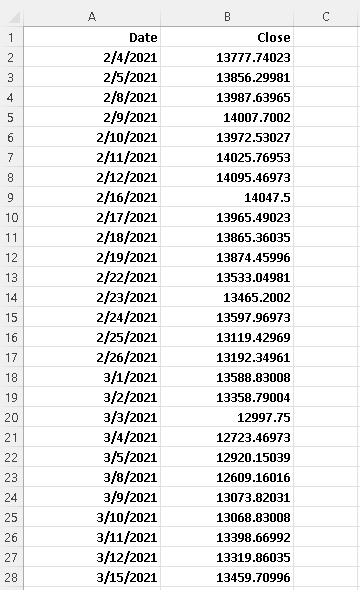
Part of the Nasdaq index values from 2/4/2021 to 2/2/2022 is shown in the table below and the whole data table is at Nasdaq Index February 2021 to February 2022
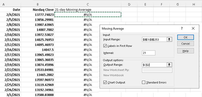
a) Use the steps in moving average using Excel to find the 21 day moving average of the Nadsaq index from 2/4/2021 to 2/2/2022 .
Solution to Example 3
Use of Excel to set up the 21 day moving average is shown below.
The graphs of the Nasdaq and its 21 day moving average are are shown below.
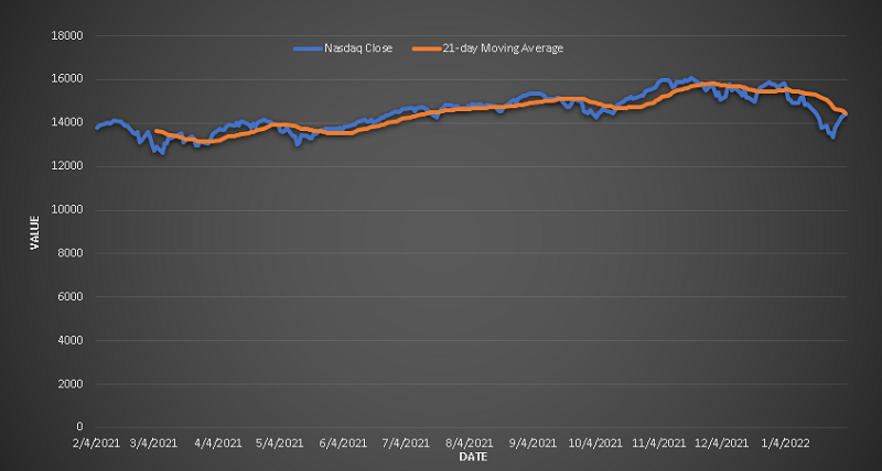
As we can see the moving average shows the overall trend over the whole period without going into the details of the daily changes.
Example 4
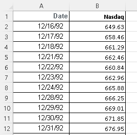
Part of the Nasdaq index values from 12/16/1992 to 2/2/2022 is shown in the table below and the whole data table is at Nasdaq Index February 1992 to February 2022
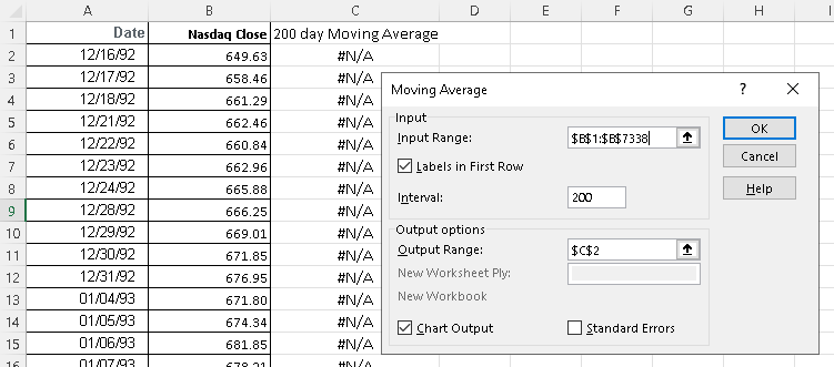
a) Use the steps in "moving average using Excel" to find the 200 day moving average of the Nadsaq index from 12/16/1992 to 2/2/2022 .
Solution to Example 4
Excel set up for 200 day moving average is shown below.
The graphs of the Nasdaq and its 200 day moving average are are shown below.
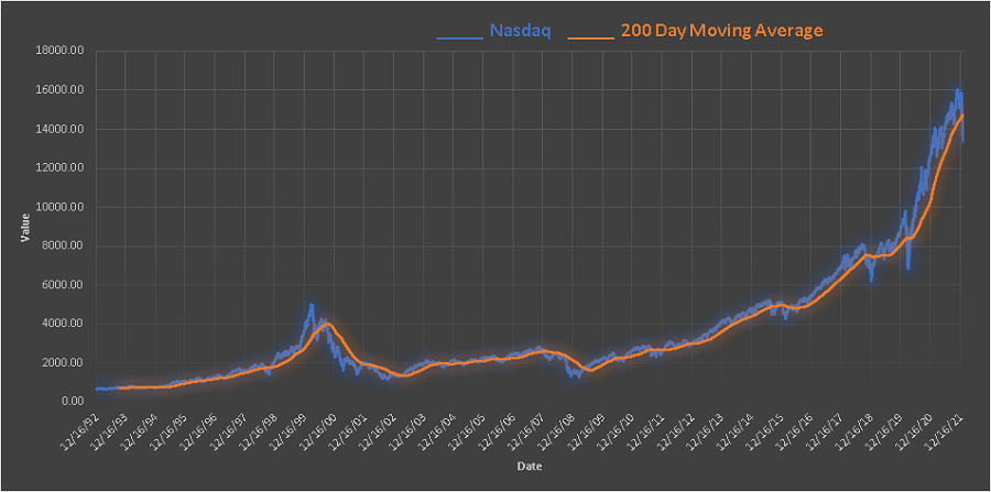
In this case, the moving average shows the overall trend over the whole period of 30 years without going into the details of the daily changes. The moving averages smooth out the graphs and are easy to read and understand the overall trend over long periods of time. They may be used to predict future trends.
More References and links
- Complete Business Statistics - Amir D. ACZEL and JAYAVEL SOUNDERPANDIAN - 6th International Edition - 2006 - ISBN 007 - 124416-6
- Solutions for Elementary Statistics a Step by Step Approach - Allan G. Bluman - 9th Edition - 2017 - ISBN-10 : 1259755339
- Complete Business Statistics - Amir D. ACZEL - 2009 - ISBN-10 : 0073373605
- Statistics - James McClave et Terry Sincich - 13th Edition - 2016 - ISBN-10 : 0134080211
- Moving Average Using Excel