Calculate Correlation Using Excel

Calculate the correlation coefficient using two different features of Excel. The first one uses the functions "f x" in Excel and the second one using the data analysis features in Excel.

1 - Calculate The Correlation Using the Functions "f x" in Excel

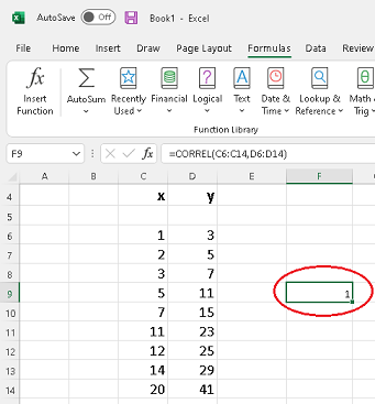
As an example, we calculate the correlation between the data set x and y already typed in two columns as shown below.
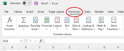
Step 1 - Select a cell anywhere near your the data.


Step 2 - Click on "Formulas" in the menu

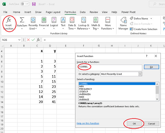
Step 3 - Click on "f x" and type (or select) "CORREL" in the window on the right, then click "OK".



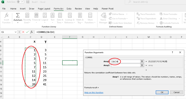
Step 4 - Clear "Array1" if necessary. Click inside "Array1" then use the mouse to select data in column 1.



Step 5 - - Click inside "Array2" and use mouse to select data in column 2 , then click OK.


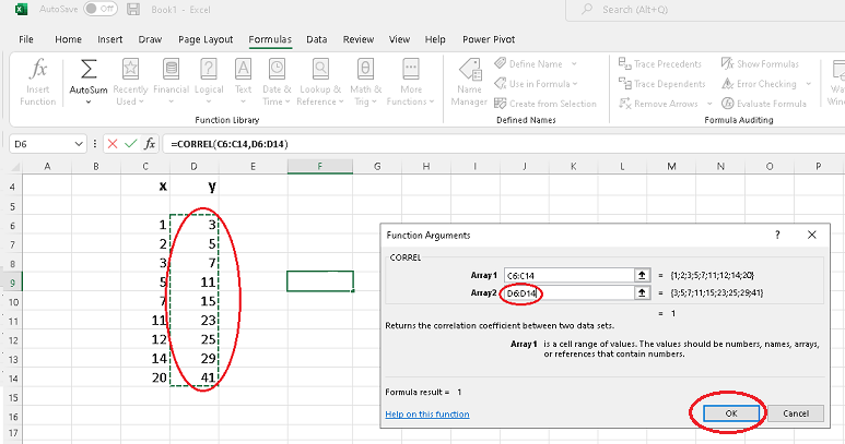
Step 6 - Read the value of the correlation coefficient, which for these data sets is equal to 1, in the cell that was selected at the start.

2 - Calculate The Correlation Using "Data Analysis" in Excel

If you are calculating the correlation of more than two data sets, it is more efficient to use the Data Analysis functions in Excel. Open your Excel file and check for the "Data Analysis" functions which should be on the right side of the menu bar. If you do not have it, you may use the steps to install it at Load The Analysis ToolPack in Excel .

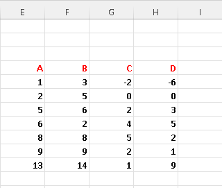
As an example, suppose that we have four data sets and we wish to calculate the correlation between the different pairs of these data sets.
Step 1 - Organize the data sets in columns and use labels in the first row such as A, B, C and D below to make it easier to read the results.


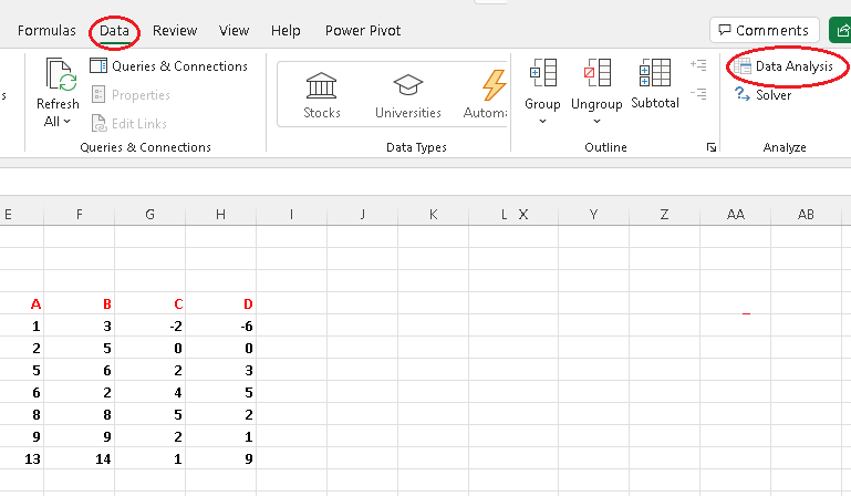
Step 2 - Press "Data" tab and click "Data Analysis".


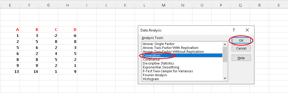
Step 3 - Select "correlation" and press "OK".


Step 4 - Clear "Input" and "Output" range.


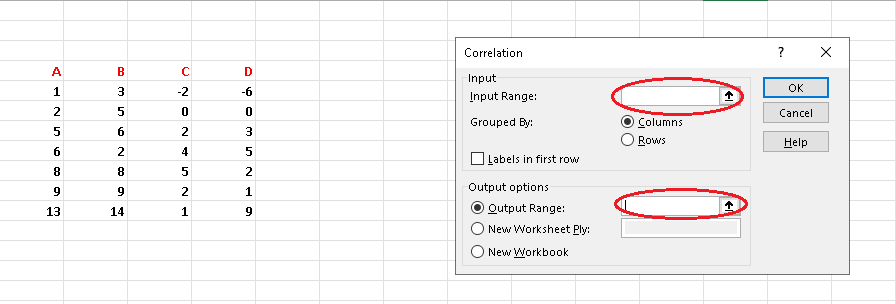
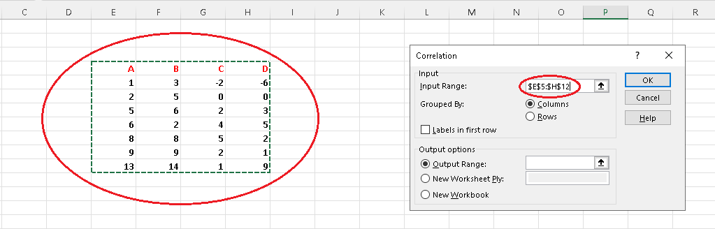
Step 5 - Use mousse and select all columns containing the data including the labels.
Note that the data may grouped by columns, which is the present case, or by rows and you need to select whichever grouping you have.


Step 6 - Check "Labels in first row" if your data has labels per column which is the case in this example. Check "Output Range" and click inside it then select a cell where you want the output to be located which in this case is cell "G18". Finally click "OK".


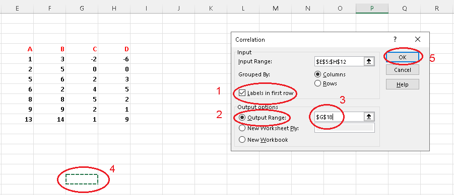
Step 7 - Read results from table: the table gives you the correlations of each pair of data.


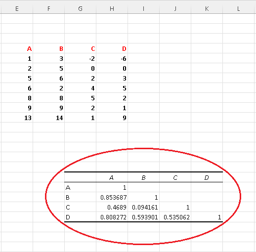
For this example, the correlation of data between column A and column A is equal to 1 shown in row A of the table of results above.
In row B, we have the correlation between data in columns B and A which is 0.853687 and the correlation between data in column B and column B which is 1.
In row C, we have the correlation between data in columns C and A which is 0.4689; the correlation between data in columns C and B which is 0.094161 and the correlation between data in column C and column C which is 1.
In row D, we have the correlation between data in columns D and A which is 0.808272; the correlation between data in columns D and B which is 0.593901; the correlation between data in columns D and C which is 0.535062, and the correlation between data in column D and D which is 1.

More References and links

1. Correlation Coefficient Examples with Solutions
2. Correlation Problems with Real Life Data
3. Load The Analysis ToolPack in Excel