Variance and Standard Deviation of a Data Set

The concpet of range , variance and standard deviation are presented along with their properties. The measure of disperion is important in statistics as it allows us to compare the variability of two or more data sets. Examples with solutions and more problems with solutions are included.

Range of a Data Set

The range of a data set is the difference between the largest and the smallest data values [1] [2] [3] [4].
Example 1
a) Find the range of and graph each data set given below. (for repeating values, arrange them vaertically)
b) Find the mean and median of each data set.
c) Compare the way the two data sets are distributed.
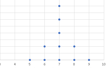
Set \(S_1\): \( \quad 2,3,4,5,6,7,8,9,10,11,12 \)
Set \(S_2\): \( \quad 5,6 , 6 , 7 , 7 , 7 , 7 , 7 , 8 , 8 , 9 \)

Solution to Example 1
a)
Set \(S_1\): Largest data value in Set \(S_1\) is equal to: 12. The smallest data value in Set \(S_1\) is equal to 2.
range = largest - smallest = 12 - 2 = 10

Set \(S_2\): Largest data value in Set \(S_2\) is equal to: 9. The smallest data value in Set \(S_2\) is equal to 5.
range = largest - smallest = 9 - 5 = 4

Clustered Data Number Line

b)
Set \(S_1\): mean = 7 , median = 7
Set \(S_2\): mean = 7 , median = 7

c)
Although the data in the sets \(S_1\) and \(S_2\) have the same mean and mode, the data in the set \(S_1\) is more dispersed (or spread out) than the data in the set \(S_2\). This is indicated by the range of \(S_1\) being larger than the range of \(S_2\). The idea of using the range to measure data disperion is not enough; we need a measure that takes into account all data values in the data set.

The Variance of a Data Set

In what follows, the odd numbered formulas are the definition formulas. The even numbered are the calculations formulas which are derived from the definition formulas but they may be more efficient to use in calculations.
The variance is the average of the sum of the squares of the distances between the data values and the mean of the data. It is a way to measure how data is distributed around the mean. A small variance means the data is closely distributed around the mean and a large variance means the data is more dispersed.

Sample

The variance of a sample is the average of the sum of the squared differences between the data values and their mean [1] [2] [3] [4].
The sample variance \( s^2 \) formula is defined by
\[ s^2 = \dfrac{\sum_{i=1}^n (x_i - \bar x)^2}{n-1} \quad (1) \]
where \( n \) is the total number of data values in the sample and \( \bar x \) the sample mean .
Note that the average is obtained by dividing the sum by \( n - 1 \) instead of \( n \).
It can be shown that the above formula ( definition ) may be written as follows
\[ s^2 = \dfrac{\sum_{i=1}^n x_i^2 - (\sum_{i=1}^n x_i)^2/n} {n-1} \quad (2) \]
which is a more practical formula since it does not need to mean \( \bar x \).

Population

The population variance \( \sigma^2 \) is defined by [1] [2] [3] [4]
\[ \sigma^2 = \dfrac{\sum_{i=1}^N (x_i - \mu)^2}{N} \quad (3) \]
where \( N \) is the total number of data values in the population and \( \mu\) the population mean .
The above formula ( definition ) may be written as follows
\[ \sigma^2 = \dfrac{\sum_{i=1}^N x_i^2 - (\sum_{i=1}^N x_i)^2/N} {N} \quad (4) \]
a more practical formula since it does not need to mean \( \sigma\).

The Standard Deviation of a Data Set

The odd numbered formulas are the definitions formulas. The even numbered formulas are the calculations formulas.

Sample

The sample standard deviation is the square root of the sample variance [1] [2] [3] [4].
\[ s = \sqrt{\dfrac{\sum_{i=1}^n (x_i - \bar x)^2}{n-1}} ) \quad (5) \]
Sample standard deviation calculation formula is given by
\[ s = \sqrt {\dfrac{\sum_{i=1}^n x_i^2 - (\sum_{i=1}^n x_i)^2/n} {n-1} } \quad (6) \]

Population

The population standard deviation is the square root of the population sample variance.
\[ \sigma = \sqrt{\dfrac{\sum_{i=1}^N (x_i - \mu )^2}{N}} \quad (7) \]
The calculation formula, obtained from the above formula, is given by
\[ \sigma = \sqrt{\dfrac{\sum_{i=1}^N x_i^2 - (\sum_{i=1}^N x_i)^2/N} {N}} \quad (8) \]

Examples and Solutions

Example 2
a) Calculate the variance using the definition and the calculations formulas of the sample data set \( 1 , -2 , 3 , 4 , 5 , 0 , -10 , 23 , 9 , 3 \).
b) Calculate the standard deviation.
b) Use Excel or any other software to calculate variance and standard deviation of the above data set and compare the results in parts a), b) and c).

Solution to Example 2
a)
There \( 10 \) data values in the given set, hence \( n = 10 \)
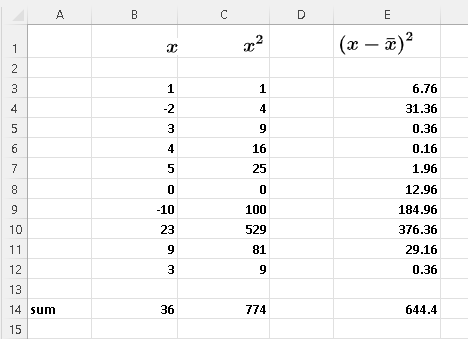
We first set up a table with columns containing the data values \( x \) and their squares \( x^2 \), B and C in this example, and their sums. We have used Excel but any software may be used.
From the table, we have
\( \sum_{i=1}^n x_i = 36 \) , \( \sum_{i=1}^n (x_i^2) = 774 \) ,
Calculate the mean: \( \bar x = \dfrac{\sum_{i=1}^10 x_i}{10} = \dfrac{36}{10} = 3.6 \)
Create a third column, E in the table below, and calculate \( (x_i - \bar x)^2 \), then the sum
\( \sum_{i=1}^n (x_i - \bar x)^2 = 644.4 \)
Table for Standard Deviation Table Calculations
Definition formula of the variance:
\( s^2 = \dfrac{\sum_{i=1}^n (x_i - \bar x)^2}{n-1} = \dfrac{644.4}{10-1} = 71.6 \)
Calculation formula for the variance
\( s^2 = \dfrac{\sum_{i=1}^n x_i^2 - (\sum_{i=1}^n x_i)^2/n} {n-1} = 71.6 \)
b)
\( s = \sqrt {s^2} = \sqrt (71.6) = 8.46167 \)
c)
Follow the step by step process in descriptive statistics using Excel to obtain the table below.
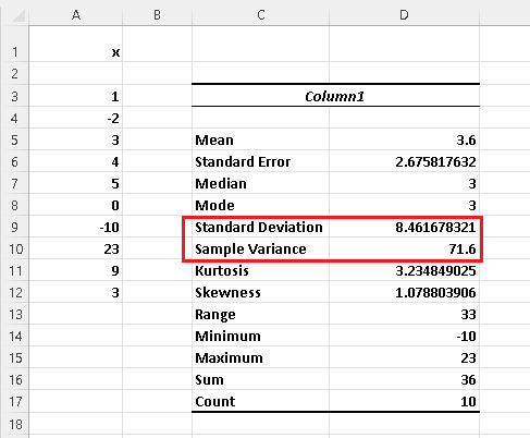
Standard Deviation Results Using Excel
Use the table above to identify:
The sample variance: \( s^2 = 71.6 \) and the sample standard deviation: \( s = 8.461678321 \).
The results obtained in parts a) and b) using the definition and calculation formulas give the same answer as the "Data Analysis" tool in Excel.

Example 3
Two data sets \(S_1\) and \(S_2\) are given below. The dispersion of these data sets was studied using the range in example 1.
Set \(S_1\): \( \quad 2,3,4,5,6,7,8,9,10,11,12 \)
Set \(S_2\): \( \quad 5,6 , 6 , 7 , 7 , 7 , 7 , 7 , 8 , 8 , 9 \)
a) Use Excel or any other software to calculate the standard deviation and variance of each of the data set of samples \(S_1\) and \(S_2\).
b) Which data has a larger standard deviation? Could this be justified from the data plot in example 1?

Solution to Example 3
a) Using the steps in descriptive statistics using Excel , we obtain the following results for the standard deviations of both sets.
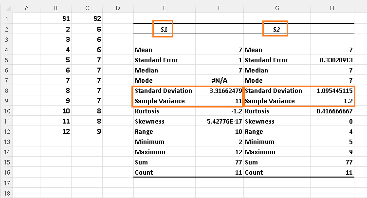
Excel Calculation Results of Standard Deviation Example 3
b) Standard deviation of \( S_1 \) is equal to 3.31662479 and the standard deviation of \( S_2 \) is equal to 1.095445115 and therefore the standard deviation of \( S_1 \) is larger.
This is justified by the data plots of \( S_1 \) and \( S_2 \) which show that the data in \( S_1 \) is more dispersed than that data in \( S_2 \).

Problems with Solutions

Problem 1
b) Plot each of the sample data sets below on a number line.
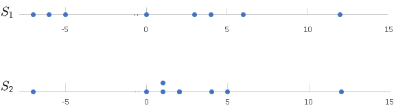
\( S_1 \) : \( -6 , 0 , 3 , 4 , - 5 , 6 , 12 , - 7 \)
\( S_2 \) : \( 1 , 2 , 2 , 12 , 0 , -7 , 4 , 5 \)
b) Find the range of each data sets.
c) Use any software to find the variance and standard deviation.
d) Which data set is more dispersed?
e) Could the answer to part d) be predicted by comparing the ranges of the data in \( S_1 \) and \( S_2 \)?
Problem 2
a) Plot the sample data sets \( S_1 \) and \( S_2 \) on a number line.
b) Find the mean of each data set.
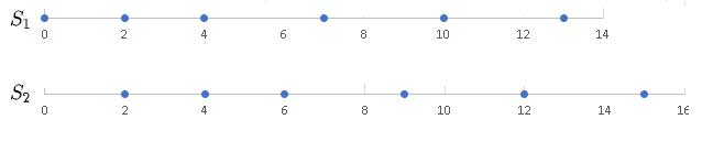
\( S_1 \) : \( 0 , 2 , 4 , 7 , 10 , 13\)
\( S_2 \) : \( 2 , 4 , 6 , 9 , 12 , 15\)
c) Examine the plots and the data distribution in the sets \( S_1 \) and \( S_2 \) and find the relationship between the data values in \( S_1 \) and \( S_2 \).
d) Find the explain why the standard deviations of the two data sets should be equal.
e) Use any software to calculate the standard deviation of each data and confirm that they are equal.

Solutions to the Above Problems

Solution to Problem 1

a)
The plots on number lines of the data in \( S_1 \) and \( S_2 \) are shown below.
Number Line Plot of Sets S1 and S2 in Problem 1
b)
\( S_1 \): Maximum data value = 12, Minimum data value = -7 , Range: \( R_1 = 12 - (-7) = 19 \).
\( S_2 \): Maximum data value = 12, Minimum data value = -7 , Range: \( R_2 = 12 - (-7) = 19 \).
c)
The steps in descriptive statistics using Excel were used to obtain the results:
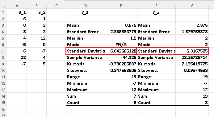
Results Standard Deviation of sets S1 and S2 Using Excel
Note that other statistics such as the mean, median, mode, range, .... are also included in the above table.
d) The standard deviation of \( S_1 \) is approximately equal to 6.64 which is larger than the standard deviation of \( S_2 \) which is approximately equal to 5.32 and therefore the data in \( S_1 \) is more dispersed that the data in \( S_2 \).
e) The ranges of both \( S_1 \) and \( S_2 \) are equal and therefore they could not be used to predict which of the data set is more dispersed.

Solution to Problem 2
The number line plots of \( S_1 \) and \( S_2 \) are shown below.
a)

Number Line Plot of Sets S1 and S2 in Problem 2
b)
Mean of \( S_1 \): \( m_1 = \dfrac{0 + 2 + 4 + 7 + 10 + 13}{6} = 6\)
Mean of \( S_2 \): \( m_1 = \dfrac{2 + 4 + 6 + 9 + 12 + 15}{6} = 8\)
c)
Examining the number line plots of \( S_1 \) and \( S_2 \), the data set \( S_2 \) is the data set \( S_1 \) shifted by two units. A closer look at the data values, reveals that we can obtain data set \( S_2 \) by adding 2 units to each data values in data set \( S_1 \).
d)
Shifting all data values in the data set does not affect the standard deviation because the mean is also shifted by the same amount, 2 units in this example, as the data values and therefore the distances between the mean do not change.
e)
Following the steps in descriptive statistics using Excel , we obtain the results:

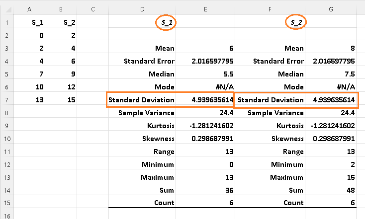
Results Standard Deviation of sets S1 and S2 Using Excel
The results in table above confirm that the variances and standard deviations of \( S_1 \) and \( S_2 \) are equal.
Note that the difference between the means and the medians of \( S_1 \) and \( S_2 \) is equal to 2 units.

Variance and Standard Deviation of a Data Set

Range of a Data Set

The Variance of a Data Set

Sample

Population

The Standard Deviation of a Data Set

Sample

Population

Examples and Solutions

Problems with Solutions

Solutions to the Above Problems

More References and links