Simple Linear Regression with Examples
\( \) \( \) \( \) \( \)
The simple linear regression model is presented with examples examples , problems and their solutions.
Examples of simple linear regression with real life data and multiple linear regression are also included.
Simple Linear Model and the Least Square
Let us assume that we have a set of ordered pairs \( (x_i , y_i) \) where \( x_i \) is the independent observed variable and \( y_i \) is the corresponding dependent observed variable with a scatter plot shown below.
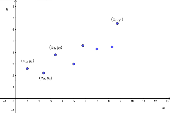
The correlation between \( x \) and \( y \) informs us on the strength of the relationship between \( x \) and \( y \), however in order to make prediction, we sometimes to go further and establish a relationship in the form of an equation betwen \( x \) and \( y \).
If the relationship between the independent observed variable \( x \) and the dependent observed variable \( y \) is close to a linear one, then the simple theoretical linear model may be written written as
\[ y = \beta_0 + \beta_1 x + \epsilon \]
\( y \) is the dependent variable that we wish to predict for values of \( x \) not included in the observed data values. \( \epsilon \) is the error or difference between the observed (or
measured) dependent variable \( y_i \) at some value of \( x_i \) and the predicted variable \( y \).
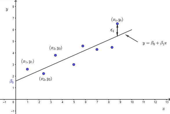
The line in the graph below is that of the linear equation \( y = \beta_0 + \beta_1 x \) whose \( y \) intercept is \( \beta_0 \) and slope \( \beta_1 \).
The graph also shows that \( \epsilon_i \) is the difference between the observed value of the dependent variable \( y_i \) and the value of \( y \) given by the equation \( y = \beta_0 + \beta_1 x \) at \( x = x_i \).
The simple theoretical linear model is valid if:
- The relationship between \( x \) and \( y \) is linear
- The errors \( \epsilon_i \) are random variables normally distributed with mean equal to zero and constant variance. Also the errors \( \epsilon_i \) are independent of each other for different observations.
Method of Least Squares for a Simple Linear Regression
So far we have dealt with a theoretical model.
Question: Given a set of observed values \( y_i \) and \( x_i \), what are the values of the y intercept \( \beta_0 \) and the slope \( \beta_1 \) that would give a good linear model as described above?
For \( m \) data points \( (x_i , y_i) \), the sum of squares of all the erros \( \epsilon_i \) is given by
\( SSE = \sum_{i=1}^{m} \epsilon_i^2 \)
with \( \epsilon_i = y_i - \hat y_i \)
where \( \hat y_i = \beta_0 + \beta_1 x_i \)
and therefore
\( SSE = \sum_{i=1}^{m} (y_i - \hat y_i )^2 = \sum_{i=1}^{m} (y_i - \beta_0 - \beta_1 x_i )^2 \)
The method of least square [1] is used to find the coefficients \( \beta_0 \) and the slope \( \beta_1 \)
From calclus [2] , \( SSE \) has a minimum value when
\( \dfrac{\partial (SSE)}{\partial \beta_0} = 0 \quad \) and \( \quad \dfrac{\partial (SSE) }{\partial \beta_1} = 0 \)
\( \dfrac{\partial (SSE)}{\partial \beta_0} = - 2 \sum_{i=1}^{m} (y_i - \beta_0 - \beta_1 x_i) \)
\(\dfrac{\partial (SSE) }{\partial \beta_1} = - 2 \sum_{i=1}^{m} x_i (y_i - \beta_0 - \beta_1 x_i) \)
which gives two equations with unknowns \( \beta_0 \) and \( \beta_1 \)
\( - 2 \sum_{i=1}^{m} (y_i - \beta_0 - \beta_1 x_i) = 0 \quad (I) \)
\(- 2 \sum_{i=1}^{m} x_i (y_i - \beta_0 - \beta_1 x_i) = 0 \quad (II) \)
Divide both sides of equations (I) and (II) by \( -2 \) and rewrite them with terms containing the unknowns \( \beta_0 \) and \( \beta_1 \) on the left.
\( \sum_{i=1}^{m} ( \beta_0 + \beta_1 x_i ) = \sum_{i=1}^{m} y_i \)
\( \sum_{i=1}^{m} (\beta_0 x_i + \beta_1 x_i) = \sum_{i=1}^{m} x_i y_i \)
Distribute the sums to obtain
\( \sum_{i=1}^{m} \beta_0 + \beta_1 \sum_{i=1}^{m} x_i = \sum_{i=1}^{m} y_i \)
\( \beta_0 \sum_{i=1}^{m} x_i + \beta_1 \sum_{i=1}^{m} x_i^2 = \sum_{i=1}^{m} x_i y_i \)
The above equations may be simplified to
\( m \beta_0 + \beta_1 \sum_{i=1}^{m} x_i = \sum_{i=1}^{m} y_i \quad (I')\)
\( \beta_0 \sum_{i=1}^{m} x_i + \beta_1 \sum_{i=1}^{m} x_i^2 = \sum_{i=1}^{m} x_i y_i \quad (I") \)
Use Cramer's rule on equations (I') and (II") to find \( \beta_1 \)
\( \beta_1 = \dfrac{m \sum_{i=1}^{m} x_i y_i - \sum_{i=1}^{m} y_i \sum_{i=1}^{m} x_i }{m \sum_{i=1}^{m} x_i^2 - (\sum_{i=1}^{m} x_i )^2} \)
Divide the numerator and denominator of the above rational expression by \( m \) to obtain
\( \beta_1 = \dfrac{\sum_{i=1}^{m} x_i y_i - \dfrac{\sum_{i=1}^{m} y_i \sum_{i=1}^{m} x_i }{m}} { \sum_{i=1}^{m} x_i^2 - \dfrac{(\sum_{i=1}^{m} x_i )^2}{m} } \)
Use equation \( (I')\) to write
\( \beta_0 = \dfrac{\sum_{i=1}^{m} y_i}{m} - \beta_1 \dfrac{ \sum_{i=1}^{m} x_i}{m} \)
Let \( \bar x = \dfrac {\sum x_i}{n} \) and \( \bar y = \dfrac {\sum y_i}{n} \) and write
\( \beta_0 = \bar y - \beta_1 \bar x \)
Sums of Squares and Cross Products
We define the sums of squares as
\( SS_x = \sum (x_i - \bar x)^2 \)
\( SS_y = \sum (y_i - \bar y)^2 \)
and the sum of cross product as
\( SS_{xy} = \sum (x_i - \bar x) (y_i - \bar y) \)
Develop and simplify \( SS_x \)
\( SS_x = \sum (x_i - \bar x)^2 = \sum (x_i^2 + \bar x^2 - 2 x_i \bar x) \\
= \sum x_i^2 + m \bar x^2 - 2 \bar x \sum x_i \\
= \sum x_i^2 + m \bar x^2 - 2 n \bar x^2 \\
= \sum x_i^2 - m \bar x^2 \\
= \sum x_i^2 - \dfrac{(\sum x_i)^2}{m} \)
Similarly, it can also be proved that
\( SS_y = \sum y_i^2 - \dfrac{(\sum y_i)^2}{m} \)
\( SS_{xy} = \sum x_i y_i - \dfrac{\sum x_i \sum y_i}{m} \)
We can now rerewrite \( \beta_1 \) and \( \beta_0 \) as
\[ \hat \beta_1 = \dfrac{SS_{xy}}{SS_{x}} \]
\[ \hat \beta_0 = \bar y - \hat \beta_1 \bar x \]
Note the symbol "hat" symbol \( \hat \cdot \) is used to indicate that \( \hat \beta_1 \) and \( \hat \beta_0 \) make the sum of errors \( \sum_{i=1}^{m} \epsilon_i^2 \) minimum.
Examples with Solutions
Example 1
Given the data in the table below,
| x | y |
|
|
| 0 | 1 |
| 2 | 5 |
| 4 | 9 |
| 5 | 11 |
| 7 | 15 |
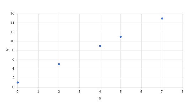
a) Use any software applications such as Google Sheets, Excel, LibreOffice .. to plot a scatter plot of y versus x.
b) Use any software applications to find the sums of squares \( SS_x \), \( SS_y \) and cross products \( SS_{xy} \)
c) Calculate the correlation coefficient \( r \)
d) Calculate \( \hat \beta_1 \) and \( \hat \beta_0 \) using the sums of squares and formulas developed above.
e) Use the equation found in part d) to calculate the value of \( \hat y \) given \( x = 2.3 \).
Solution Example 1
a)
Excel was used to make a scatter plot of "average page engaged time (y)" versus the total "average pageview duration (x)" as is shown below.
b)
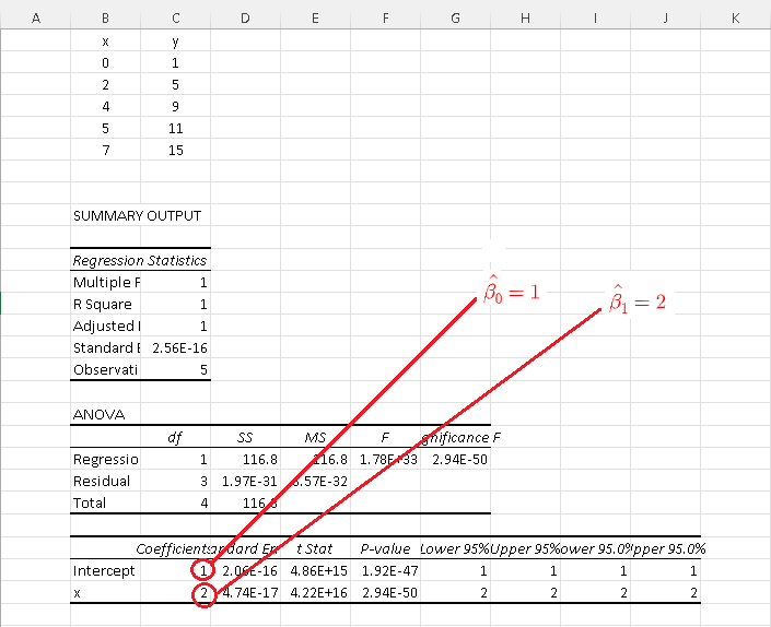
There are 5 pairs of data values \( (x_i,y_i) \), hence \( m = 5 \).
Excel was also used to do all the calculations of sums (red):
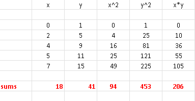
From the above table, we have
\( \sum x_i = 18 \) , \( \sum y_i = 41\) , \( \sum x_i y_i = 206\),
\( \sum x_i^2= 94\) , \( \sum y_i^2= 453\)
We now use the sum of squares formulas to write
\( SSx = \sum x_i^2 - \dfrac{(\sum x_i)^2}{m} \\
=
94 - \dfrac{18^2}{5} = \dfrac{146}{5} \)
\( SS_y = \sum y_i^2 - \dfrac{(\sum y_i)^2}{m} \\
= 453 - \dfrac{41^2}{5} = \dfrac{584}{5} \)
\( SS_{xy} = \sum x y - \dfrac{\sum x \sum y}{m} \\
= 206 - \dfrac{18 \times 41}{5} \\
= \dfrac{292}{5}
\)
c)
The correlation coefficient between \( x \) and \( y \) is given by
\( r = \dfrac{SSxy}{\sqrt {SSx \cdot SSy}} \\
= \dfrac{\dfrac{292}{5}}{\sqrt { \dfrac{146}{5} \cdot \dfrac{584}{5} }} \\
= 1 \)
d)
We now use the formulas for \( \hat \beta_1 \) and \( \hat \beta_0 \)
\( \hat \beta_1 = \dfrac{SS_{xy}}{SS_{x}} \\
\quad = \dfrac{\dfrac{292}{5}}{\dfrac{146}{5} } \\
\quad = 2
\)
\( \hat \beta_0 = \bar y - \hat \beta_1 \bar x \\
\quad = \dfrac{\sum y_i}{ 5} - \hat \beta_1 \times \dfrac{\sum x_i}{ 5}\\
\quad = \dfrac{41}{5} - 2 \times \dfrac{18}{5} \\
\quad = 1
\)
e)
Our regression model above is given by
\( \hat y = \hat \beta_1 x + \hat \beta_0 = 2 x + 1\)
Substitute by its numerical value 2.3
\( \hat y = 2 \times 2.3 + 1 = 5.6 \)
Example 2
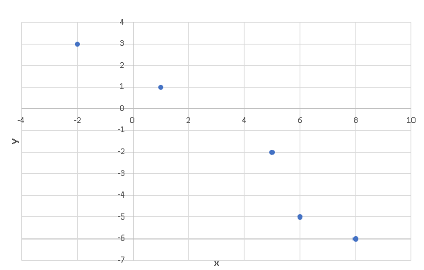
Given the data in the table below,
| x | y |
|
|
| -2 | 3 |
| 1 | 1 |
| 5 | - 2 |
| 6 | -5 |
| 8 | - 6 |
a) Use any software applications such as Google Sheets, Excel, LibreOffice .. to plot a scatter plot of y versus x.
b) Use any software applications to find the sums of squares \( SS_x \), \( SS_y \) and cross products \( SS_{xy} \)
c) Calculate the correlation coefficient \( r \).
d) Calculate \( \hat \beta_1 \) and \( \hat \beta_0 \) using the sums of squares and formulas developed above.
e) Use the equation found in part d) to calculate the value of \( \hat y \) given \( x = 1.5 \).
Solution Example 2
a)
Excel was used to make a scatter plot of "average page engaged time (y)" versus the total "average pageview duration (x)" as is shown below.
b)
There are 5 pairs of data values \( (x_i,y_i) \), hence \( m = 5 \).
Excel was also used to do all the calculations of sums (red):
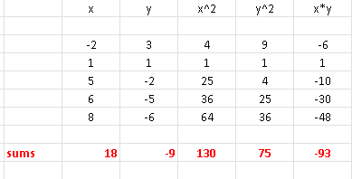
\( \sum x_i = 18\) , \( \sum y_i = -9 \),
\( \sum x_i y_i = -93\) , \( \sum x_i^2= 130\) , \( \sum y_i^2= 75\)
\( SSx = \sum x_i^2 - \dfrac{(\sum x_i)^2}{m} \\
=
130 - \dfrac{18^2}{5} = \dfrac{326}{5} \)
\( SS_y = \sum y_i^2 - \dfrac{(\sum y_i)^2}{m} \\
= 75 - \dfrac{(-9)^2}{5} = \dfrac{294}{5} \)
\( SS_{xy} = \sum x y - \dfrac{\sum x \sum y}{m} \\
= -93 - \dfrac{ 18 \times (-9)}{5} \\
= -\dfrac{303}{5}
\)
c)
The correlation coefficient between \( x \) and \( y \) is given by
\( r = \dfrac{SSxy}{\sqrt {SSx \cdot SSy}} \\
= \dfrac{-\dfrac{303}{5}}{\sqrt { \dfrac{326}{5} \cdot \dfrac{294}{5} }} \\
= -0.97872 \)
d)
Using the formulas for \( \hat \beta_1 \) and \( \hat \beta_0 \) to obtain
\( \hat \beta_1 = \dfrac{SS_{xy}}{SS_{x}} \\
\quad = \dfrac{-\dfrac{303}{5}}{ \dfrac{326}{5} } \\
\quad = -0.92944
\)
\( \hat \beta_0 = \bar y - \hat \beta_1 \bar x \\
\quad = \dfrac{\sum y_i}{ 5} - \hat \beta_1 {\sum x_i}{ 5}\\
\quad = \dfrac{-9}{5} + 0.92944 \dfrac{18}{5} \\
\quad = 1.545984
\)
e)
The regression model is given by
\( \hat y = \hat \beta_1 x + \hat \beta_0 \)
Substitute \( \hat \beta_1 , \hat \beta_0 \) and \( x \) by their numerical values
\( \hat y = -0.92944 \times 1.5 + 1.545984 = 0.151824 \)
Example 3
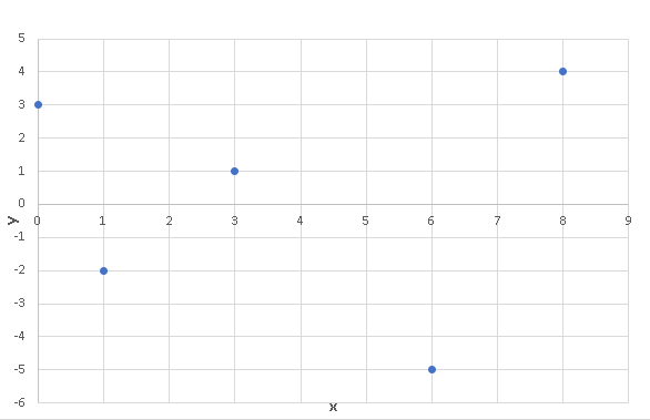
Given the data in the table below,
| x | y |
|
|
| 0 | 3 |
| 1 | -2 |
| 5 | 1 |
| 6 | -5 |
| 8 | 4 |
a) Use any software applications such as Google Sheets, Excel, LibreOffice .. to plot a scatter plot of y versus x.
b) Use any software applications to find the sums of squares \( SS_x \), \( SS_y \) and cross products \( SS_{xy} \)
c) Calculate the correlation coefficient \( r \).
d) Examine the scatter plot and the correlation; is a linear regression an appropriate model for the given data?
Solution Example 3
a)
Excel was used to make a scatter plot of "average page engaged time (y)" versus the total "average pageview duration (x)" as is shown below.
b)
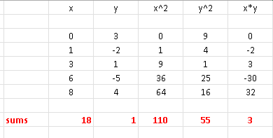
There are 60 pairs of data values \( (x_i,y_i) \), hence \( m = 5 \).
Excel was also used to do all the calculations of sums (red):
\( \sum x_i = 18\) , \( \sum y_i = 1\),
\( \sum x_i y_i = 3\) , \( \sum x_i^2= 110\) , \( \sum y_i^2= 55\)
\( SSx = \sum x_i^2 - \dfrac{(\sum x_i)^2}{m} \\
=
110 - \dfrac{18^2}{5} = \dfrac{226}{5} \)
\( SS_y = \sum y_i^2 - \dfrac{(\sum y_i)^2}{m} \\
= 55 - \dfrac{1^2}{5} = \dfrac{274}{5} \)
\( SS_{xy} = \sum x y - \dfrac{\sum x \sum y}{m} \\
= 3 - \dfrac{ 18 \times 1}{5} \\
= -\dfrac{3}{5}
\)
c)
The correlation coefficient between \( x \) and \( y \) is given by
\( r = \dfrac{SSxy}{\sqrt {SSx \cdot SSy}} \\
= \dfrac{-\dfrac{3}{5}}{\sqrt { \dfrac{226}{5} \cdot \dfrac{274}{5} }} \\
= -0.01205 \)
d)
The scatter plot shows that there is no linear relationship between x and y. This is also confirmed by the value of the correlation coefficient \( r \) calculated above and is close to zero. Hence the linear regression model is not appropriated for the given data.
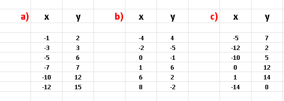
Example 4
The data sets in examples 1 and 2 above are shown in the tables below,
a)
| x | y |
|
|
| 0 | 1 |
| 2 | 5 |
| 4 | 9 |
| 5 | 11 |
| 7 | 15 |
(b)
| x | y |
|
|
| -2 | 3 |
| 1 | 1 |
| 5 | - 2 |
| 6 | -5 |
| 8 | - 6 |
Use Excel to calculate the coefficients involved in the simple linear regression
of each data set and compare the results to those obtained in examples 1 and 2.
Note that you may use any other software applications such as Google Sheets, LibreOffice to do the above calculations.
Solution Example 4
a)
The results of calculations using Excel for data set a) are shown below and the simple linear model is given by:
\( \hat y = \hat \beta_1 x + \hat \beta_0 = 2 x + 1 \)
The above results are exactly what was found in example 1 above.
The results for data set b) are shown below and the simple linear model is given by:
\( \hat y = \hat \beta_1 x + \hat \beta_0 = - 0.929448 x + 1.546012 \)
The above results are close to the results \( \hat y = -0.92944 \times x + 1.545984\) found in example 2 above.
You may use the online multiple linear regression calculator to check answers to the examples and problems.
Problems with Solutions
Problem 1
For each data set below,
A) make a scatter plot,
B) calculate the correlation coefficient using Excel or any other software applications such as Google Sheets, LibreOffice ...
C) Calculate the Coefficient of Determination using Excel or any other software applications.
D) decide which data set(s) may be appropriately modelled using simple linear regression model and find \( \hat \beta_0 \) and \( \hat \beta_1 \) using Excel or any other software applications such as Google Sheets, LibreOffice...
Problem 2
Given the data set below,
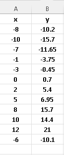
A) make a scatter plot,
B) calculate the correlation coefficient using Excel or any other software applications such as Google Sheets, LibreOffice ...
C) Use Excel to determine the coefficients \( \hat \beta_0 \) and \( \hat \beta_1 \) involved in the linear regression.
D) Use the linear regression model to predict the value of \( y \) for \( x = 1.02 \)
Solutions to the Above Problems
Solution to Problem 1
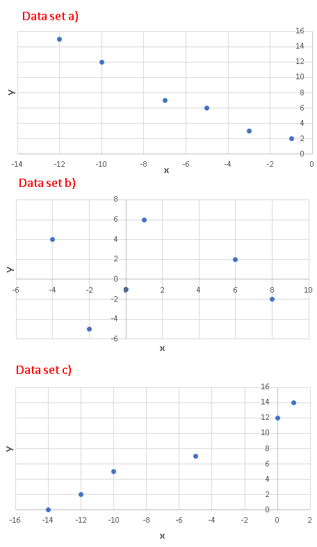
A)
The scatter plots of each data set is shown below
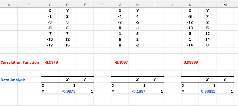
B)
The correlation of each dataset is shown below and calculated using Excel "Correlation Function"(red) and Excel "Data Analysis" tools(blue).
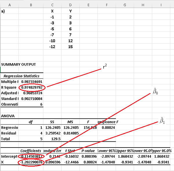
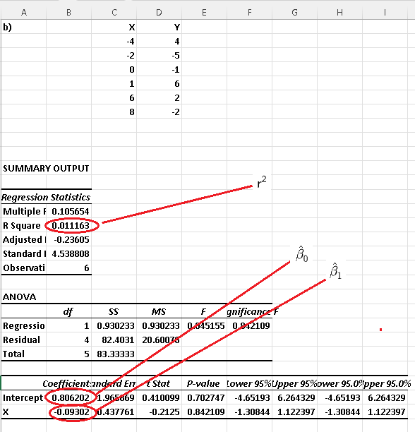
C)
Using Excel for simple linear regression to each dataset, we obtain the following results where \( r^2 \) is the coefficient of determination.
D)
In part D) above we found the correlation coefficients and we can deduce that absolute values of the correlations of datasets a) and c) are close to 1. Also their factors of determination \( r^2 \) are also close to 1. In fact we can check that, for each dataset, the square of the correlation coefficient is equal to the coefficient of determination.
Hence both datasets a) and c) may be modeled using a linear regression model. Both the correlation and the coefficient of determination of the dataset c) are close to zero and therefore a linear regression model for this data set would not be a good one.
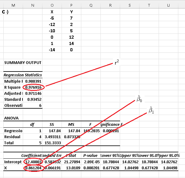
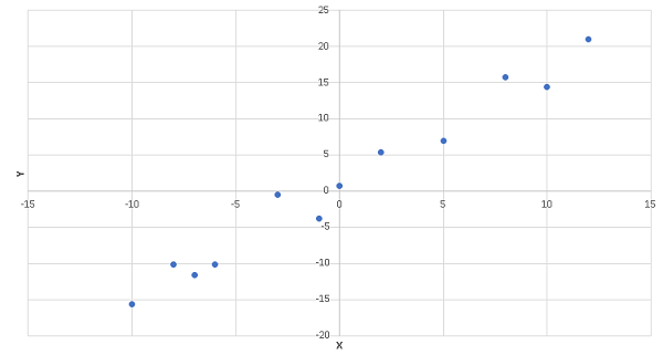
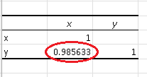
Solution to Problem 2
A)
The scatter plots of each data set is shown below
B)
Using Excel, the correlation is given by
C)
The use of Excel gives the following results
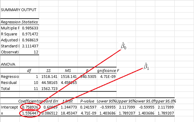
D)
\( \hat y = \hat \beta_1 x + \hat \beta_0 \\
1.596447 x + 0.758926 \)
Substitute \( x \) by its numerical value \( 1.02 \)
\( \hat y = 1.596447 \times 1.02 + 0.758926 = 2.38730194 \)
More References and links
- Mansfield Merriman, "A List of Writings Relating to the Method of Least Squares"
- University Calculus - Early Transcendental - Joel Hass, Maurice D. Weir, George B. Thomas, Jr., Christopher Heil - ISBN-13 ? : ? 978-0134995540
- Coefficient of Determination
- Simple Linear Regression Examples with Real Life Data
- Correlation Coefficient
- Simple Linear Regression Using Excel
- Multiple Linear Regression Using Excel
- Multiple Linear Regression Calculator